Roger Chen and Sarah Kim
For our final project, we chose to do 3 projects: the Tour into the Picture, Video Textures, and High Dynamic Range imaging.
The tour into the picture method creates a 3-dimensional world using a single 2-dimensional image that has single-point perspective. This works by assuming the scene of the image can be modeled as a box. 5 sides of the box are visible. By labeling the vanishing point and the sides of the box in the image, we can extrapolate world coordinates for each of the 5 planes and then use 3D rendering techniques to explore the image.
We decided to implement our Tour into the Picture with WebGL and CoffeeScript, so that it could run in the web browser. The following demos are not videos, they are rendered directly in the browser.
Here is a demonstration of our WebGL Tour into the Picture running in fully automatic guided mode. In this example, we move the camera toward the rear plane while rotating it slightly (we move the Euler angles in a small circle as we progress down the hallway).
You can also control the WebGL Tour into the Picture yourself using the keyboard or button clicking. First, choose an input image (the image plane parameters have been pre-selected for you), and then use either the buttons or the arrow keys to move through the scene.
Choose an image to view:
When you select an image above, an interactive tour GUI will appear here in your web browser.
We created a GUI for labeling Tour into the Picture data points. This helps us gather the TIP parameters in a visual way, instead of trying to pick out points in Photoshop. The GUI provides:
You can upload an image to the GUI and label it. The GUI outputs JSON data that can be used in many programming languages. You can also just try out the GUI by following this link:
The GUI also displays the Tour into the Picture WebGL code so you can explore your newly labeled TIP image.
In case your browser is too old to use any of the previous demos, we have pre-rendered some examples of our TIP code in action.
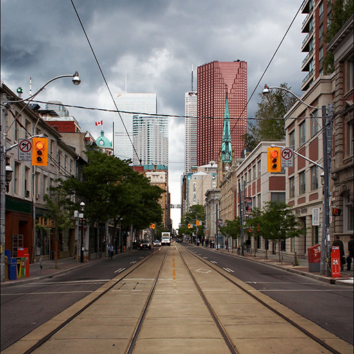
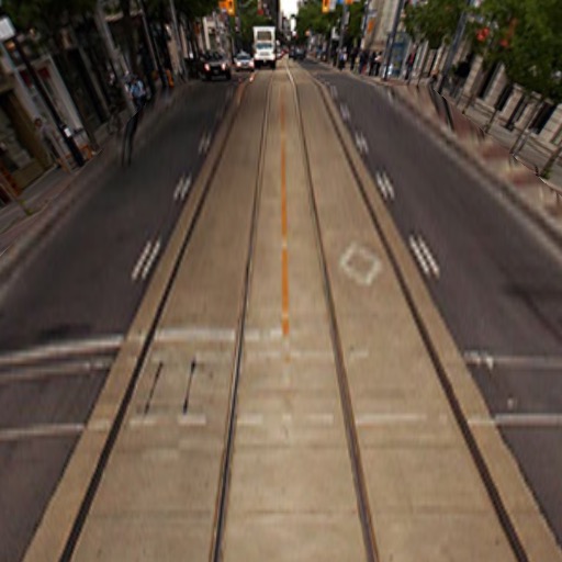
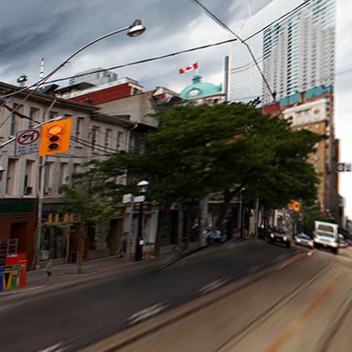
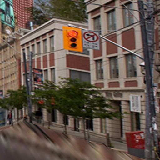
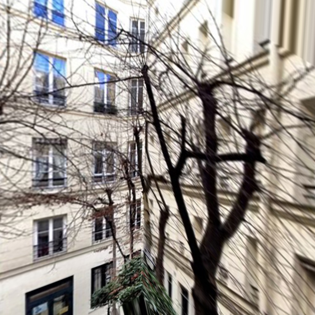
This city example doesn’t exactly fit into the assumptions of 1-D perspective, since the cars and trees stick out. I chose to use the building facades as the left and right wall. The ceiling is not very well defined, because the sky is the ceiling, but I just chose the highest building. The back plane is also not very well defined either. Nonetheless, I can get some interesting views out of this example.
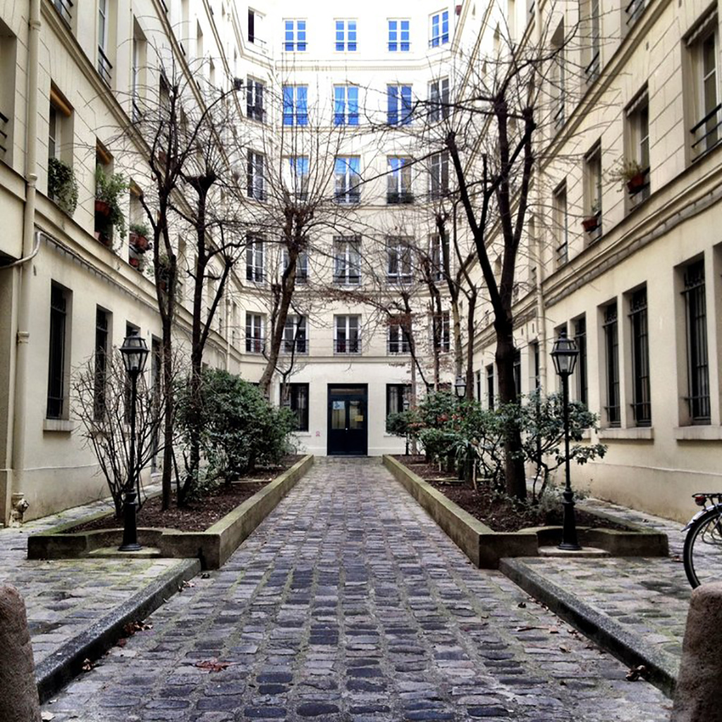
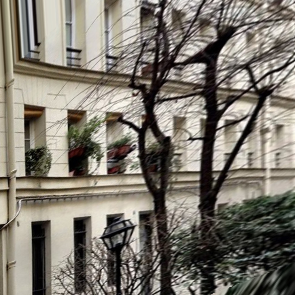
This courtyard example works much better, since the geometry is simpler. However, the planters in the center still mess up the 1-D perspective assumptions.
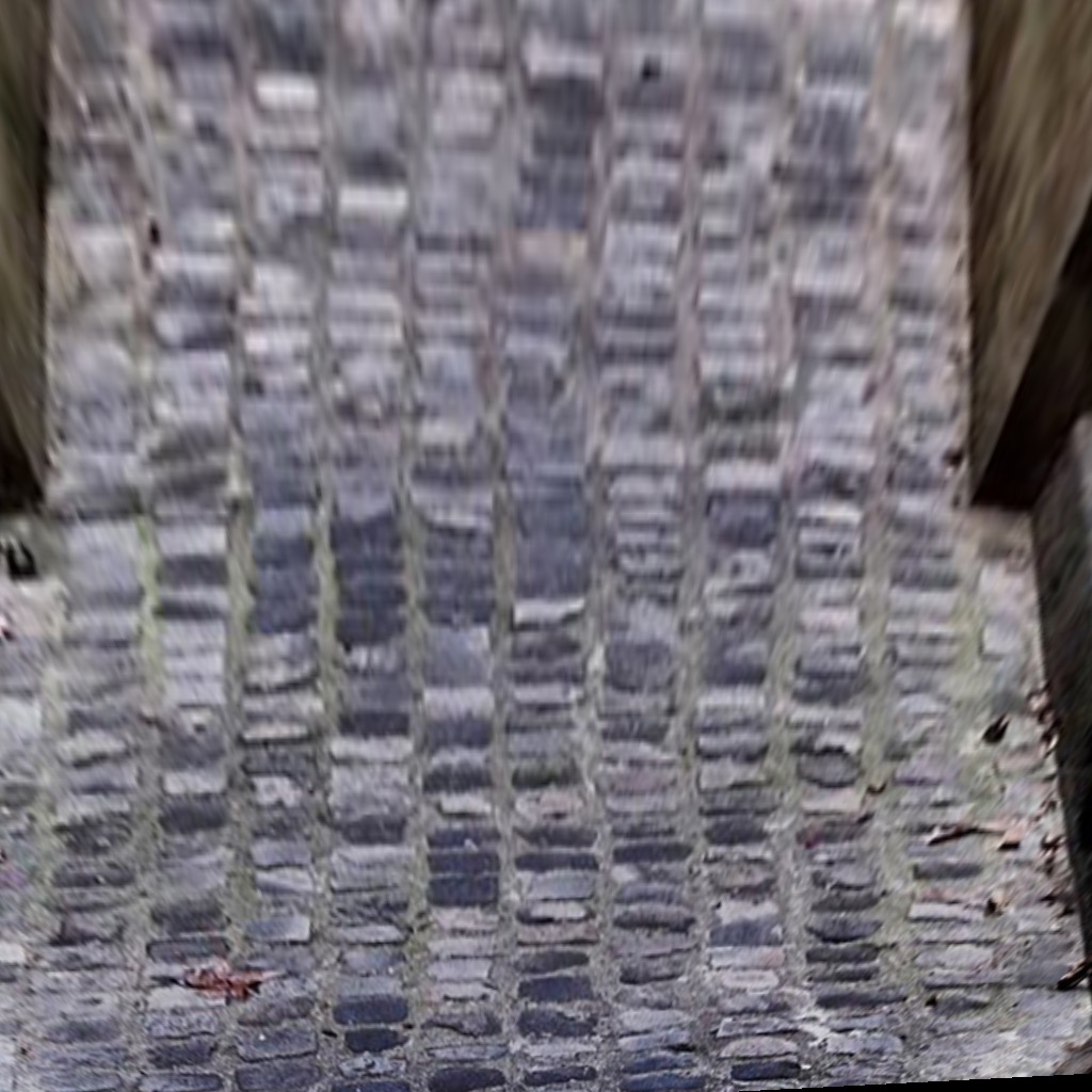
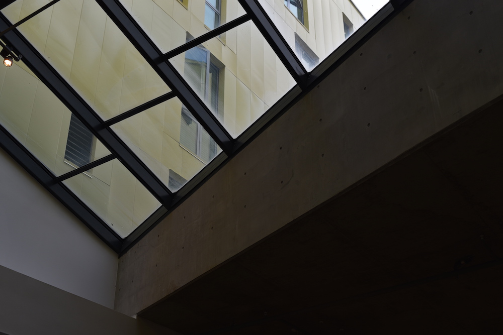
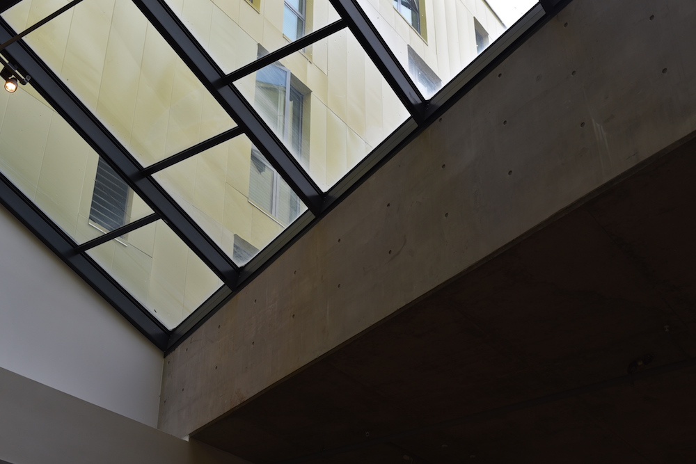
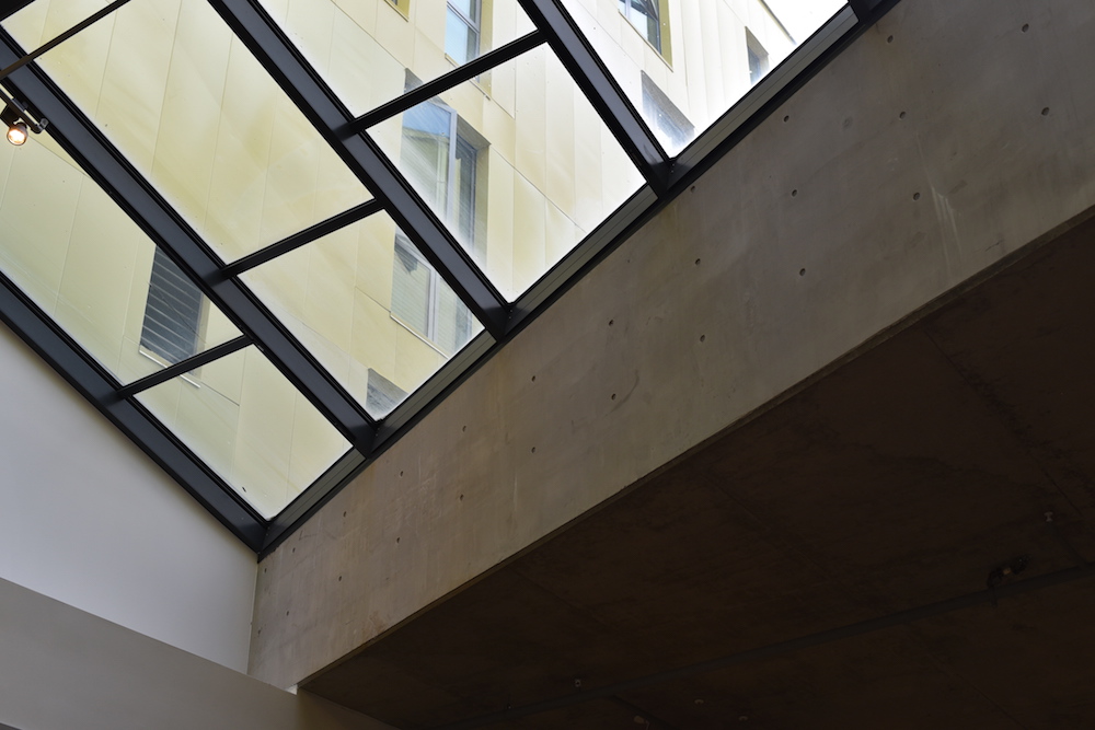
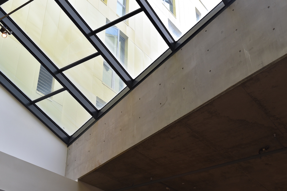
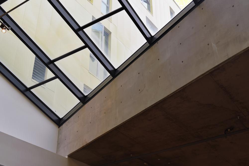
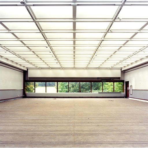
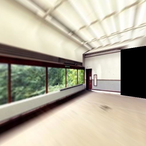
This museum is probably the best example, since the room is empty and the walls and ceiling are very straight. However, I wish that there were more pixels devoted to the left and right walls. In the 3-D model, the left and right walls are very short as a result.
The goal of the video textures method is to synthesize a video of arbitrary length, given a small clip of “training” video. It is a video texture, because like image textures, video textures look the best when transitions are seamless.
We decided to implement our video textures with OpenCV and C++. The OpenCV framework takes care of video decoding/encoding and also provides fast matrix libraries. Our final program can render video textures in real-time as well as generate video clips and save them to a file.
An infinite video texture can be represented with 1) the original set of frames from the training video, and 2) a 2D transition model matrix where Ti,j represents the probability that frame j will follow frame i−1. This implies that the last frame is a dead end, because there are no entries in the transition model for it. We compute this transition model matrix with the following steps:
Each frame of the video is first extracted and then reduced to 1/4th of its original size on each dimension. The downsampling was done to speed up computation time, since video frames have a lot of noise anyway.
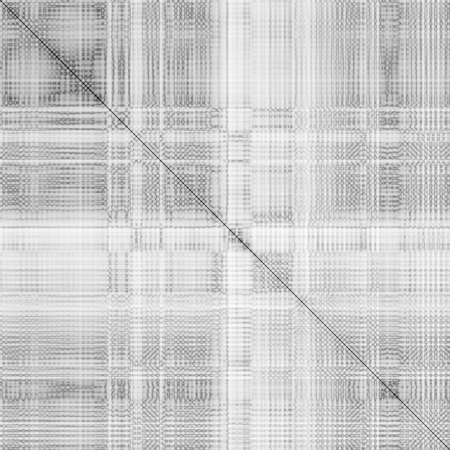
We create a N × N matrix (where N is the number of total video frames) that contains the L2 distance between each frame and each other frame. We call this matrix D. This is a symmetric matrix, so we only need to compute half the values and then just copy them across the diagonal. The values on the diagonal are always 0.
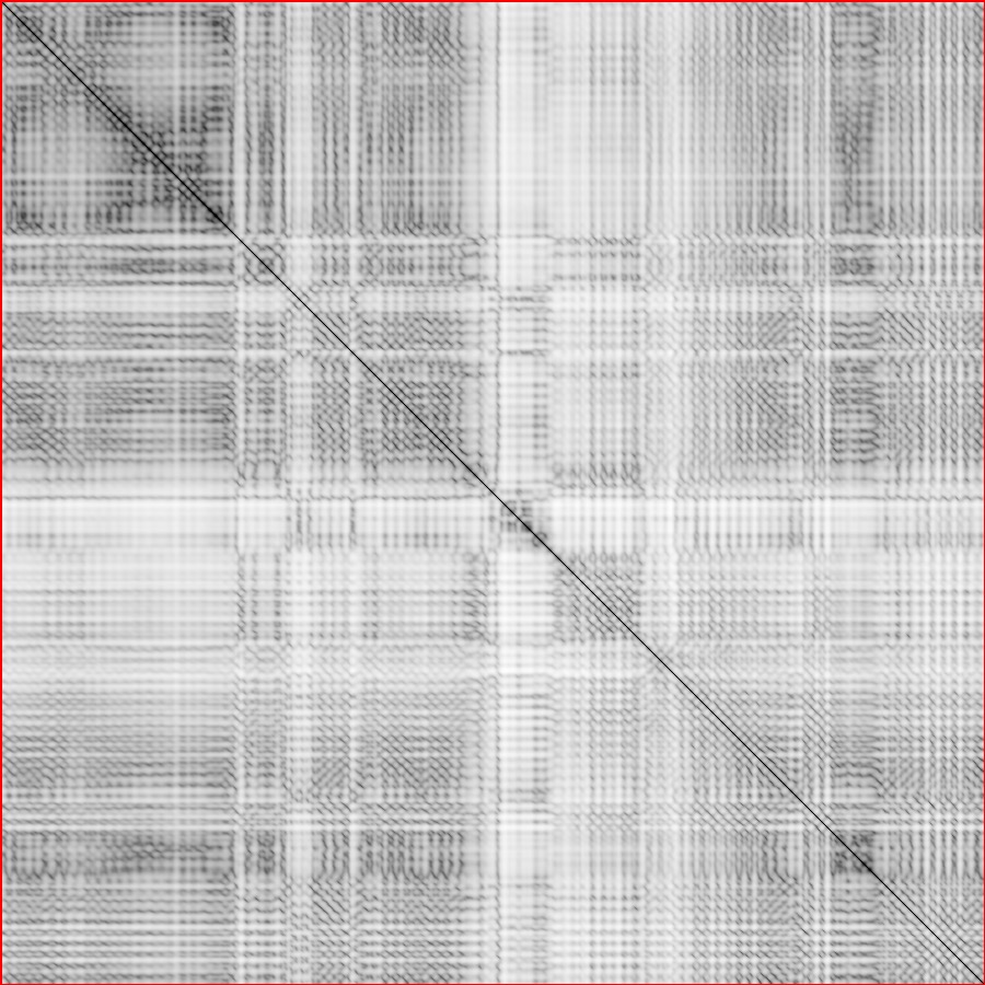
As described in the original video textures paper, we apply a filter over the values of D so that distances don’t only consider the difference between 2 frames, but also their neighboring frames. We use a binomial weight distribution with m = 2 (2 frames before, and 1 frame after). Here is the formula used:
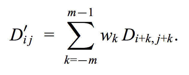
We call this new matrix D′. This new matrix discards the first 2 frames and the last 1 frame, because when we apply the filter, they do not have enough frames before/after them to fully compute the distance.
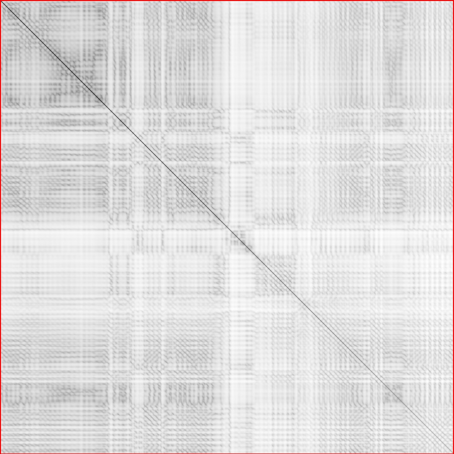
When the video texture reaches the last valid frame (frame N), it can no longer try to find a good frame to continue the playback. Therefore, when the program is currently displaying frame N - 1, it must always jump backward to a different point in the video, and never to frame N. In general, we can label frame N as off-limits, because it is a dead end. We use the following definition to define a new matrix D″ to capture this idea.
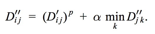
Because this definition is recursively defined, we must iterate through the matrix and update its elements in a loop until they converge. We used the method in the paper to do this efficiently. I defined the stopping condition to be when the sum of the non-infinite values of the min() expressions is below a certain epsilon. The value of epsilon is defined to be the initial sum of the non-infinite values of the min() expression, divided by 10.
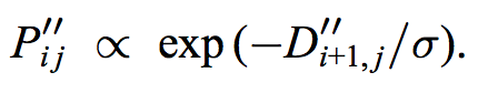
We apply the following formula to turn our distance matrix D″ into a probability matrix. The values are normalized such that every row adds up to 1, unless there are infinite values in the row (for the off-limit frames). Our value of sigma is set to be the average non-infinite distance value, divided by 27 (determined heuristically to be a pretty good choice).
We suppress transitions that have a neighbor which has a higher probability than the current transition. However, we leave the main diagonal alone, in order to avoid frames that have no possible remaining transitions. We normalize each row to sum up to 1 again after this operation.
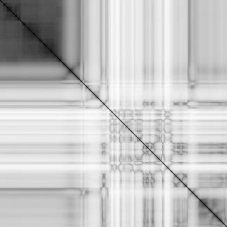
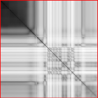
This is our final transition model. Here is a visualization of each step in the derivation process for a particular video that exhibits very strong periodicity (spoiler: it’s a pendulum).


Each of these examples contains a source video (left) and a synthesized video (right). The synthesized video has an overlay that displays the most recent jumps (jumps of +1 frame are ignored, because they are the most common) as well as the current frame’s position in the source image.
The original paper used a candle video as an example, so I started out with that. The nice thing about a candle is that there is essentially only 1 dimension to its motion. That dimension is how far left or right the candle is blowing. In this particular video, the candle starts out very still, and then it flickers. This property can be seen in the visualization of the transition model.
The upper left region corresponds to the region where the candle is still. In this case, the candle tends to jump back to another stationary frame, so the candle remains still. The lower left region corresponds to the frames toward the end where the flame is flickering. In the lower left region, we have a lot of frames that potentially could jump back to the beginning of the video, because of our dead-end avoidance.
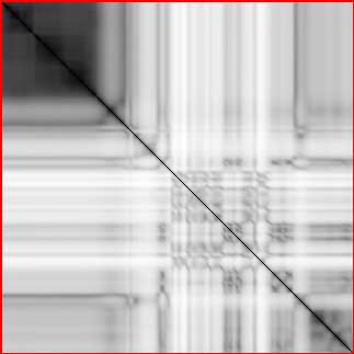
The pendulum video is periodic, so we get a nice pattern in our transition model. However, you can see that before we apply “Preserving dynamics”, the forward and reverse jumps have an equal amount of weight, which means the pendulum can suddenly change the direction of its velocity, which does not look natural. After preserving dynamics, the jumps that correspond to the opposite direction are attenuated. (The effect is not as noticeable in the visualization of the distance matrix, because we take the logarithm of its values before rendering the visualization. However, you can easily see the effect of preserving dynamics after the inverse exponentiation step.
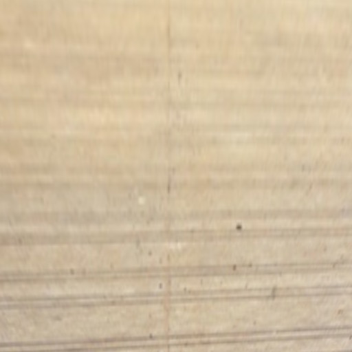
This flower video benefited greatly from the non-maximal suppression step. The background of this flower video is constantly changing and adds a lot of noise to the transition model. However, non-maximal suppression is able to pick out the best transition points despite the noise and minimize how much discontinuity appears in the blurred background.
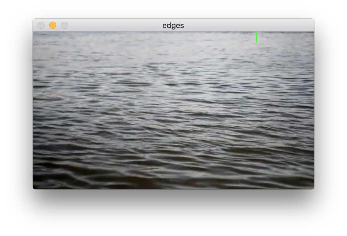
This was the most difficult input video. I thought that water texture would be easy at first, but there is a very visible discontinuity where the video jumps back to the beginning, because a video of water has very high dimensionality to it. All of the water waves can be in different positions, and it is very difficult to find two unrelated frames that actually look similar.


Our video textures application also runs as a GUI. It displays the same visualization as the rendered video. It can save and load the transition matrix to/from a file, so that it does not have to be recomputed every time.
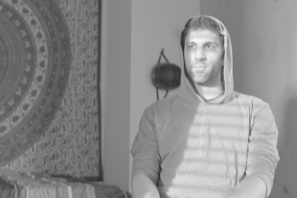
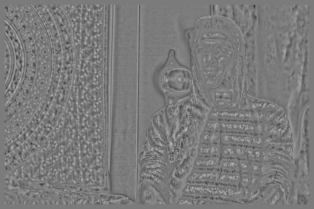
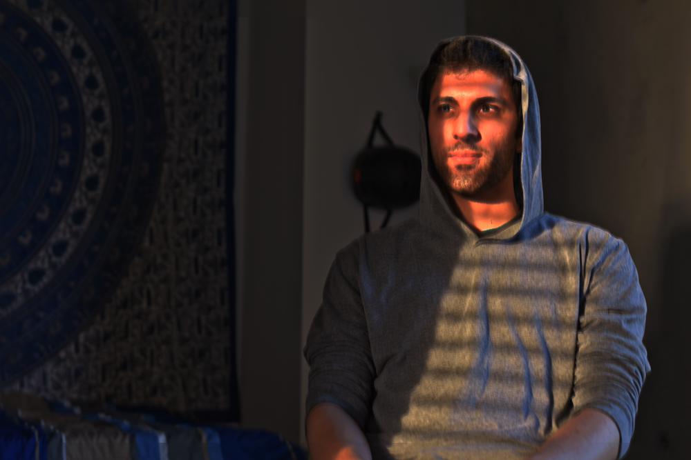
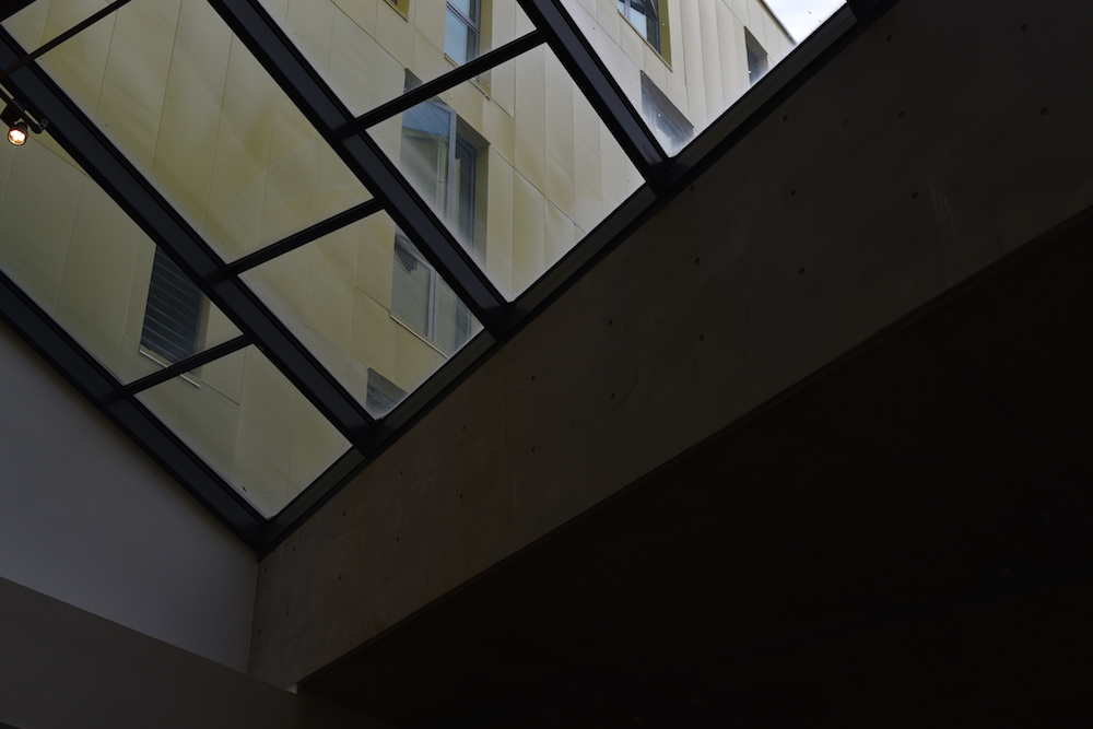
The real world has a very large dynamic range that cannot be simultaneously fully captured by cameras. The goal of HDR is to determine the radiance of a scene from multiple exposures and remap this radiance onto pixel values to attempt to more fully express the range of the original scene with a limited number of values.
HDR is composed of two separate steps: (1) constructing a radiance map of relative intensity values of scene locations and (2) applying tone operators to map the radiance map to the small range of [0, 255] pixel values.
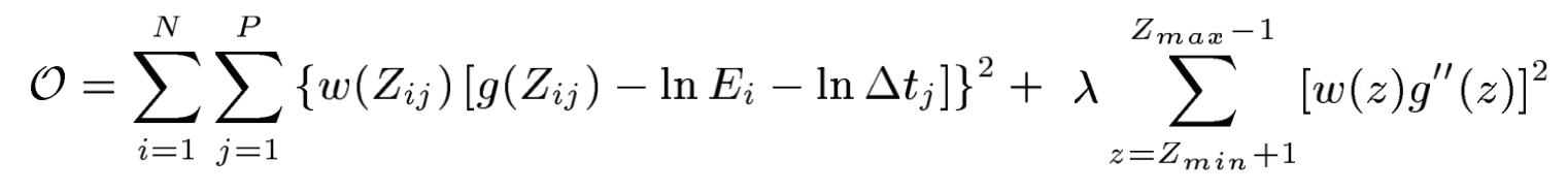
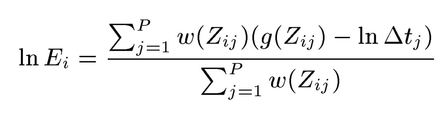
This algorithm was taken from Debevec and Malik 1997. Recovering the radiance map of a scene is composed into several steps:
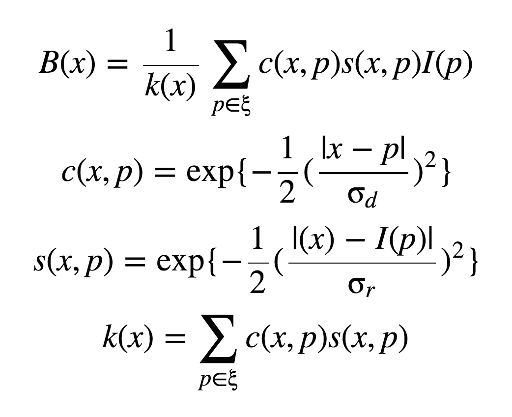
Once we have radiance values, it is necessary to find the proper mapping from the large spread of values to the limited [0, 255] pixel value range. We worked on two different tone mappers:

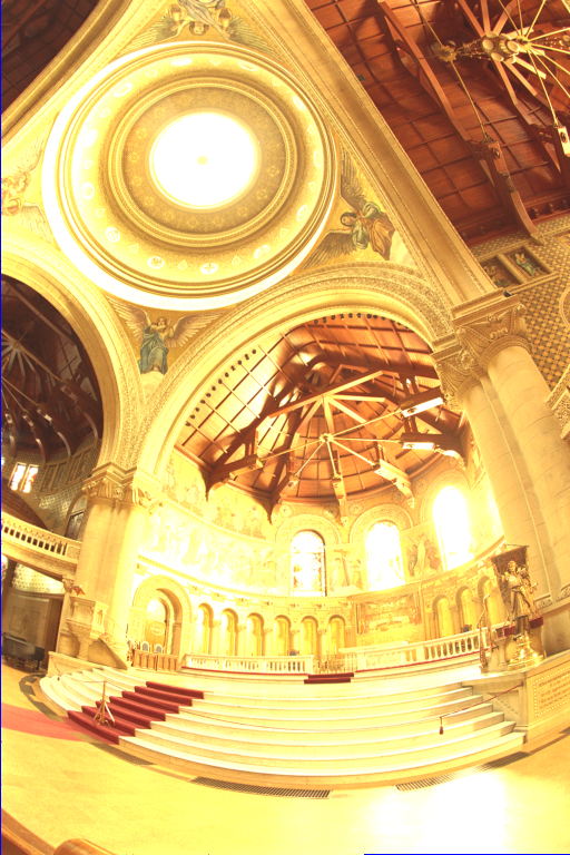
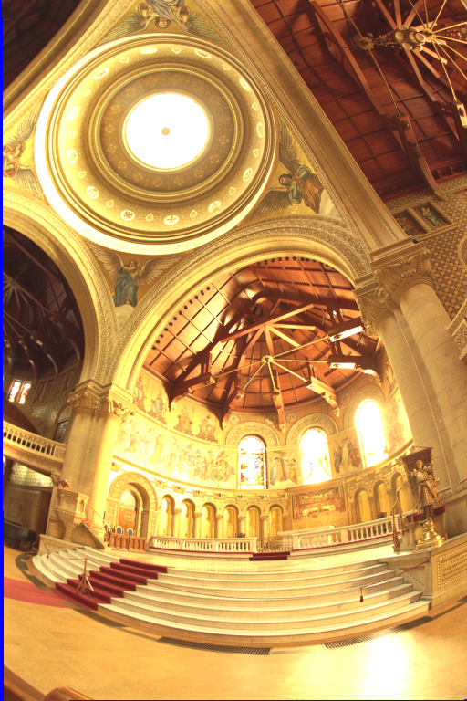
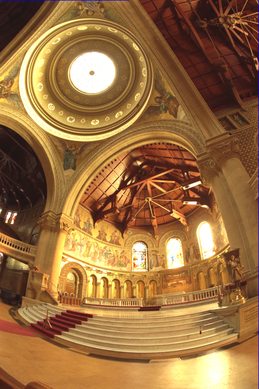
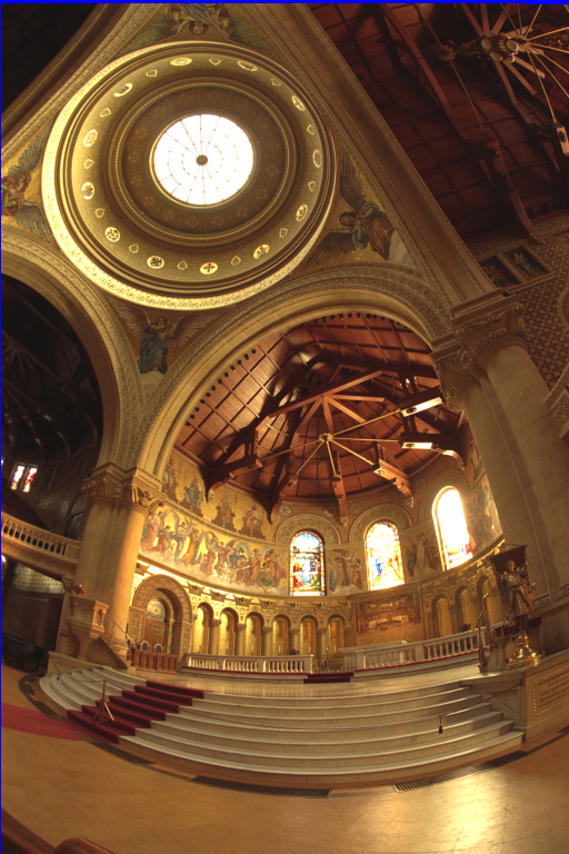
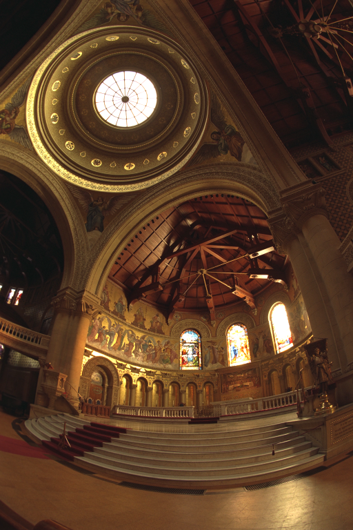
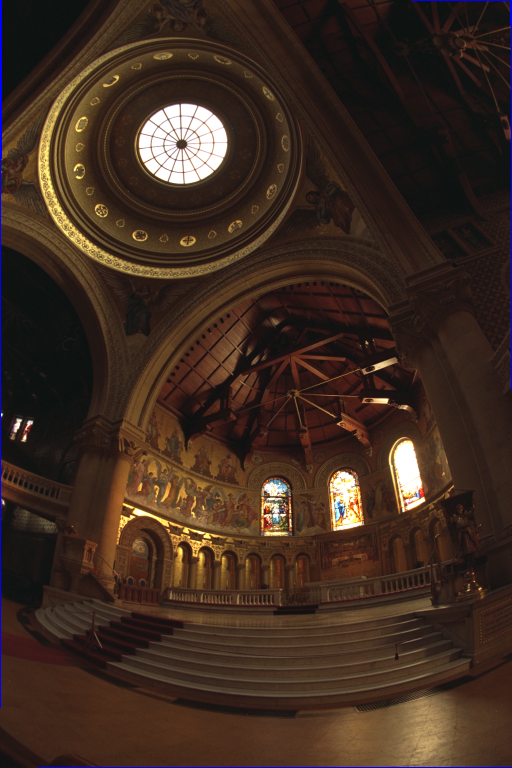
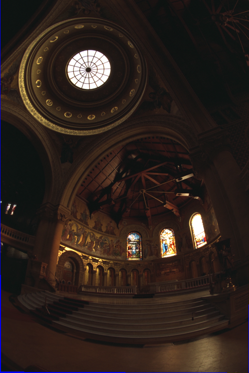
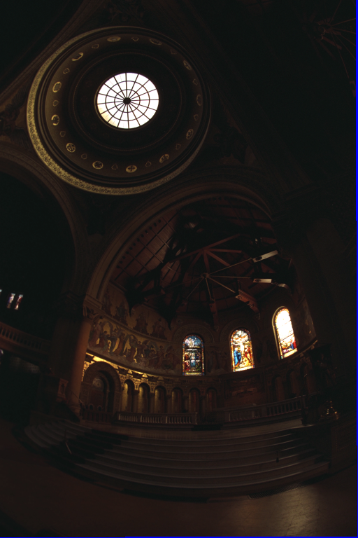
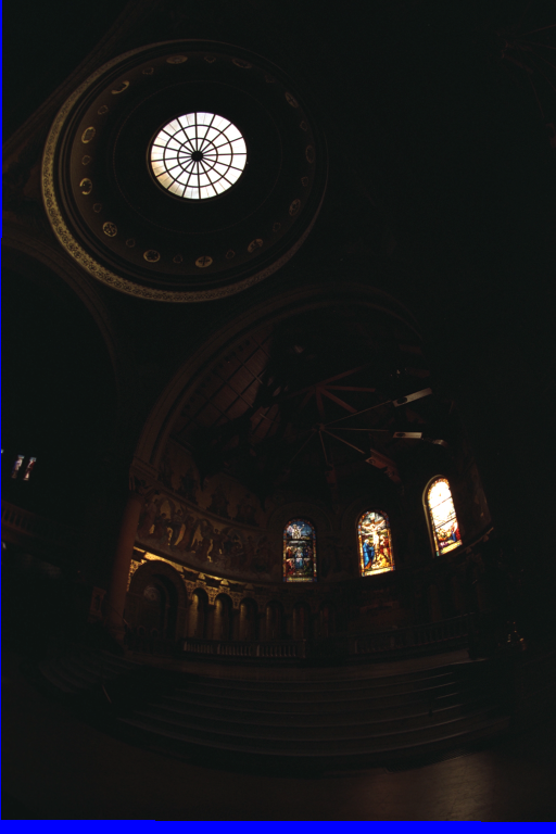
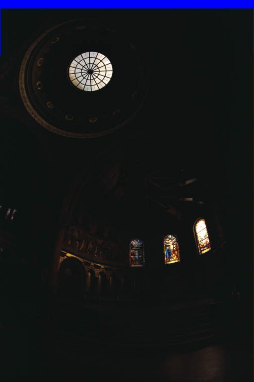
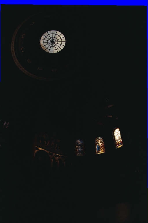
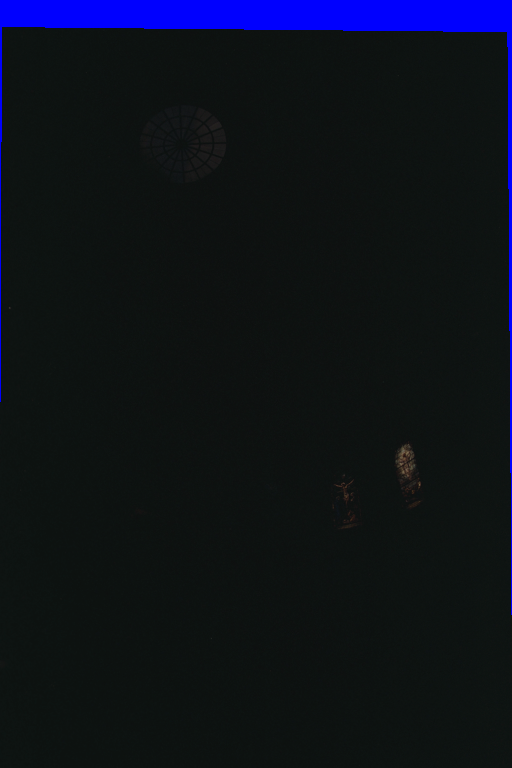
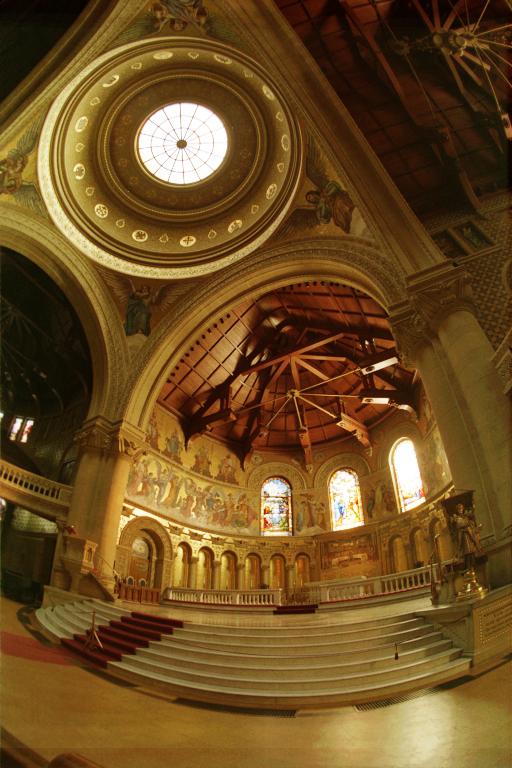
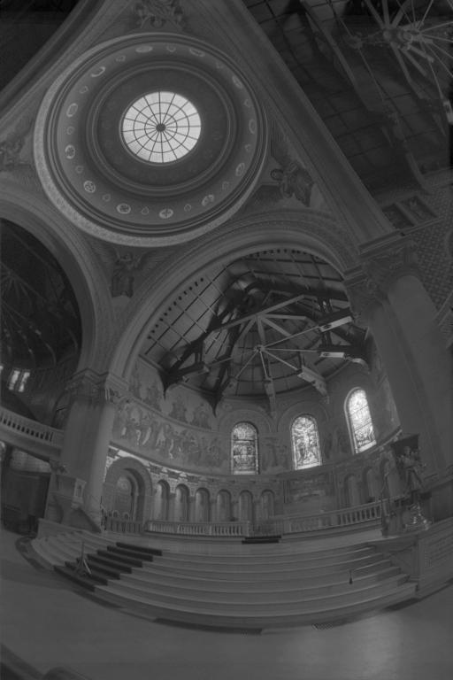
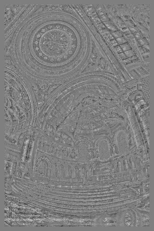
This set of images of Stanford Memorial Church (source) is the classic example used by both Debevec and Durand.
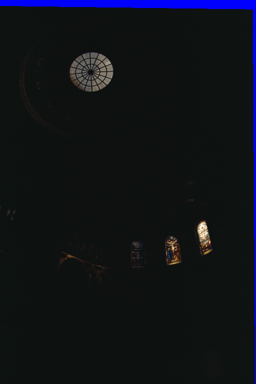
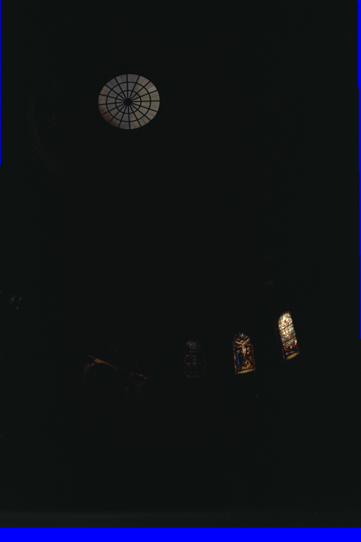
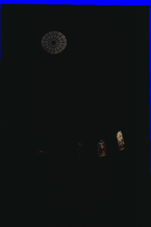
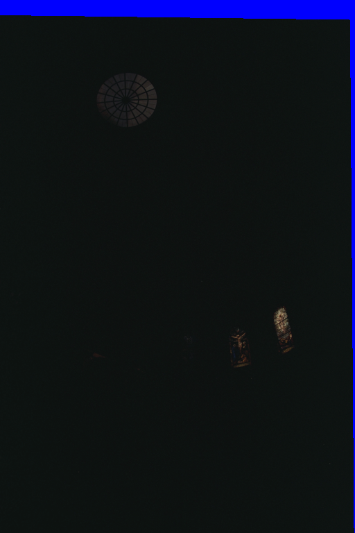
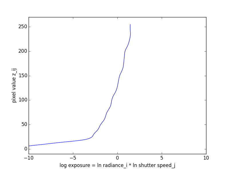
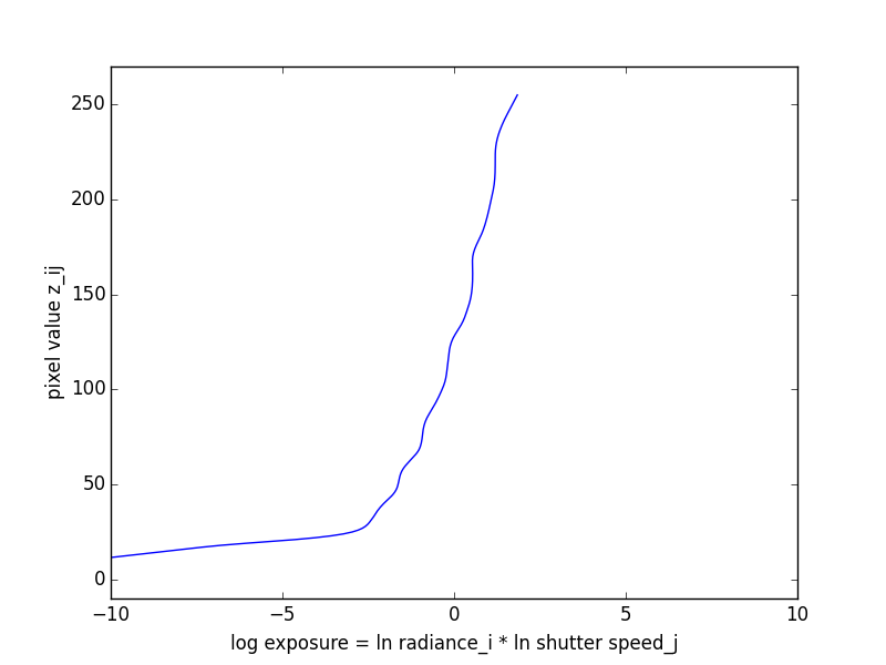
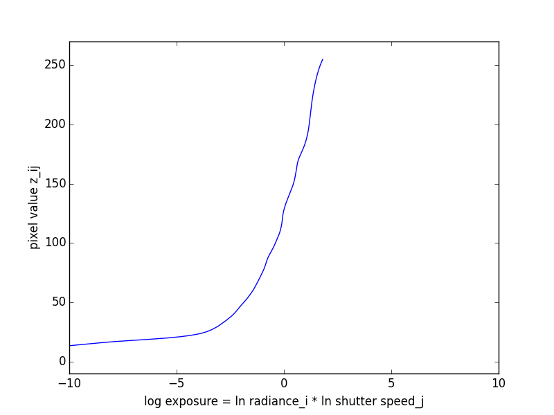
Here are the recovered response curves for the three channels.
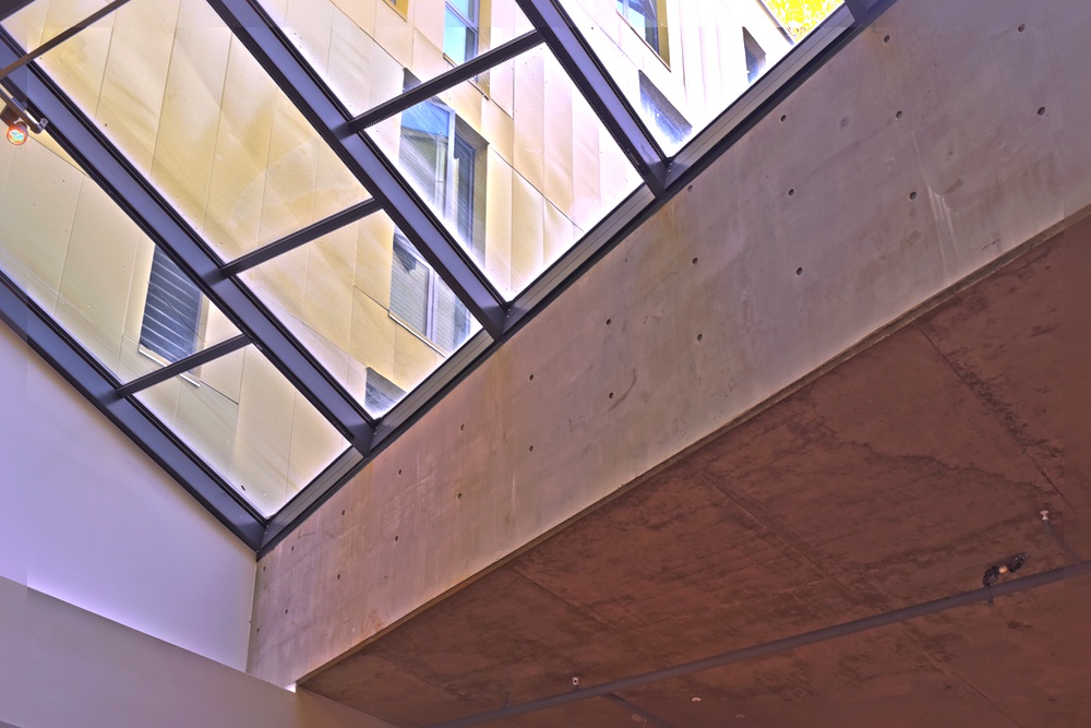
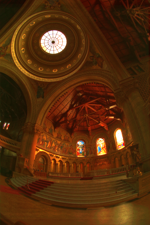
Of the left side of the row of images below is the result of applying the global Reinhart tone mapper. On the right side is the result of the applying the local Durand tone mapper.
Here are the results of HDR on some of our own pictures!