
Roger Chen
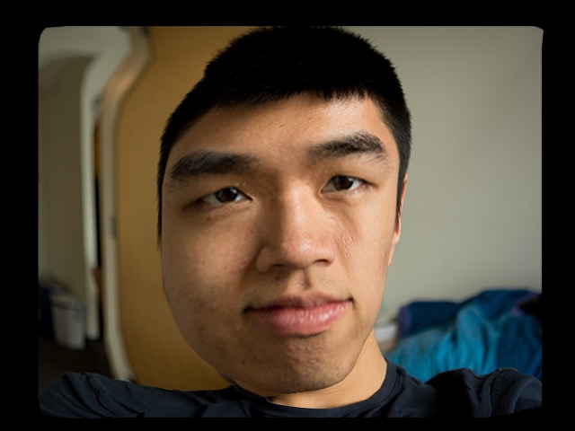
In this assignment, images of faces are blended and morphed, by both their texture and their shape. This was accomplished by first annotating the location of keypoints in the source images. The keypoints on faces determine the position of the eyes, nose, mouth, eyebrows, cheeks, and other important features of the face.
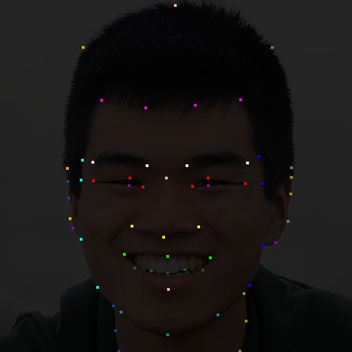
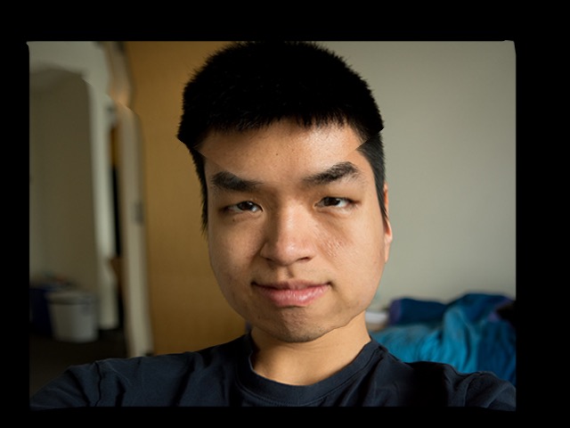
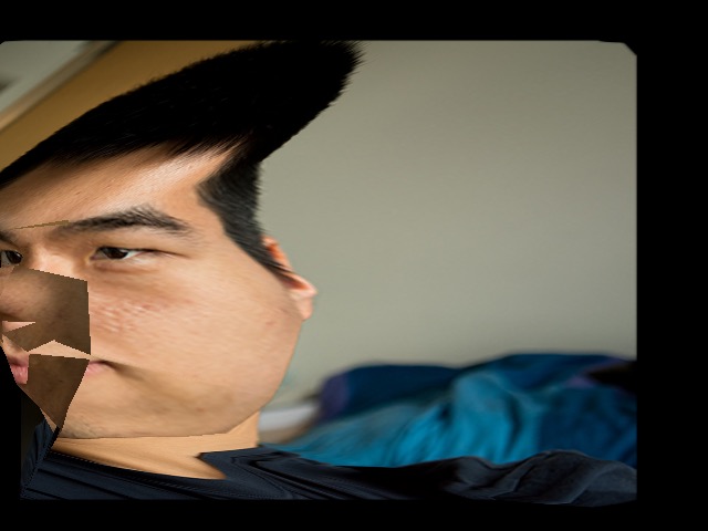
I wanted to be able to label keypoints in the most intuitive way possible, without having to tweak numbers or duplicate any work. I also wanted to use my existing tools as much as possible, rather than build my own interface for labeling. So, I labeled my keypoints in Adobe Photoshop as colored 1x1 pixel dots on a black canvas, which has the same dimensions as the original image.
However, simply labeling points not enough, unless we know which points in image 1 correspond to which points in image 2. Therefore, I divide my labeled points into multiple series. Each series contains all the points of a particular color. The points in a series are either ordered vertically (by their y component) or horizontally (by their x component), depending on which dimension has greater variance among the points of that series. Finally, all of the series are sorted by the hex values of their colors, which ensures a consistent ordering between different images.
In the example, each color is a different series. The horizontal magenta series defines the hairline. The vertical cyan series defines the outline of the face’s right cheek. (The actual keypoints image has a black background and the points are 1x1, not 4x4.)
I also added the 4 corners of each image to the list of keypoints. This is useful, because we can always assume that the entire image is contained within the convex hull of the keypoints.
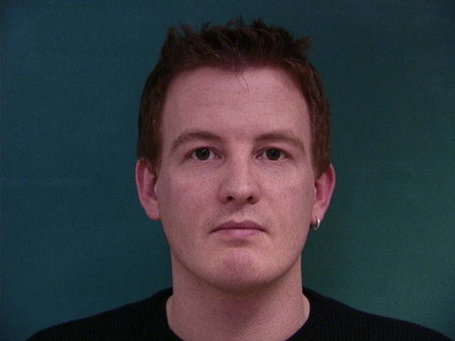
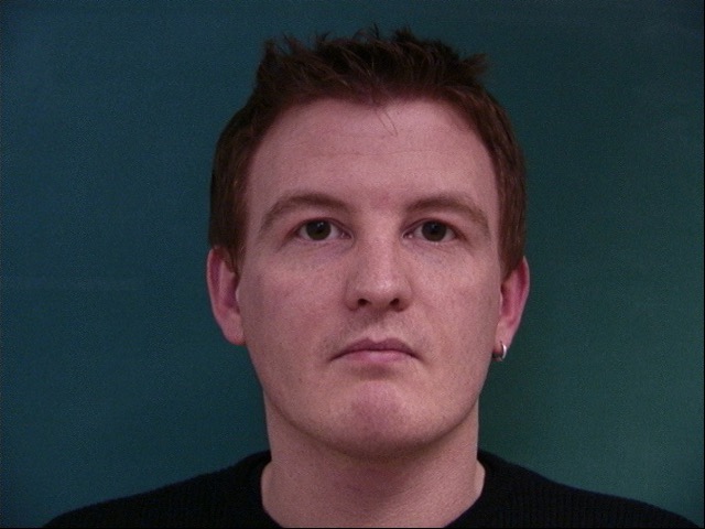
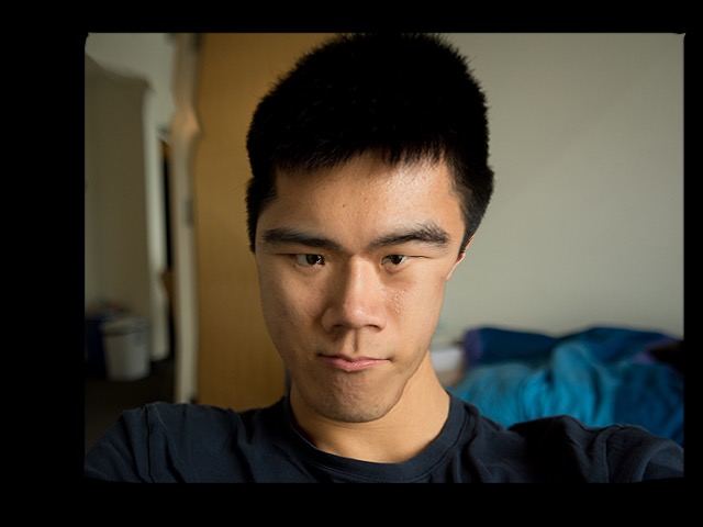
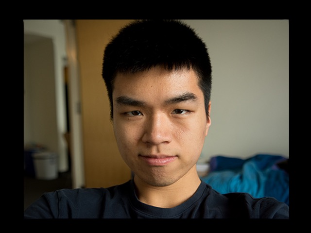
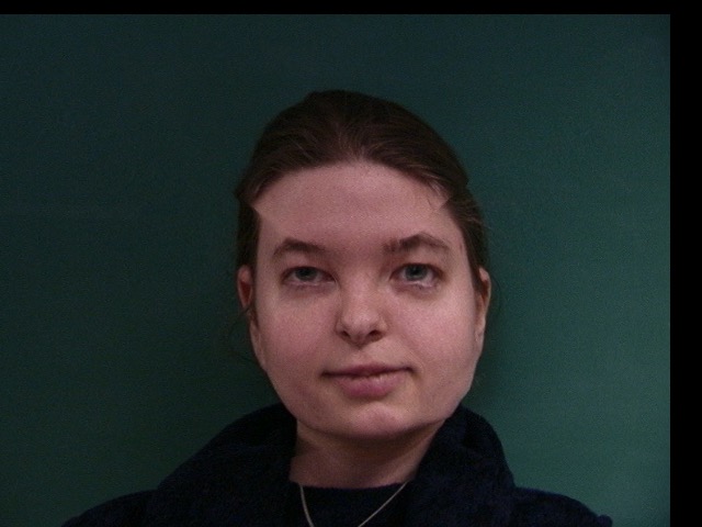
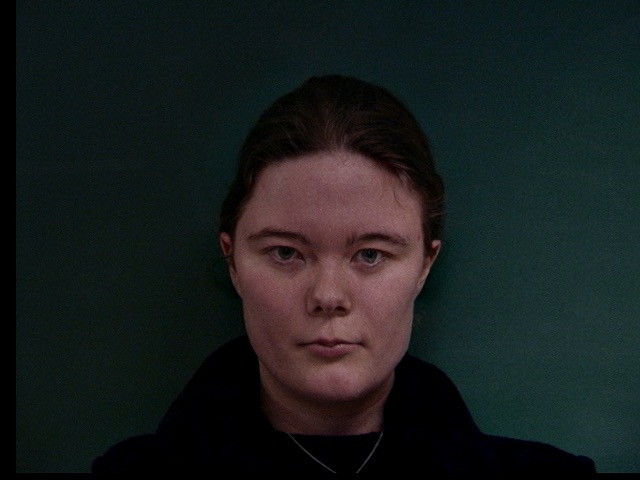
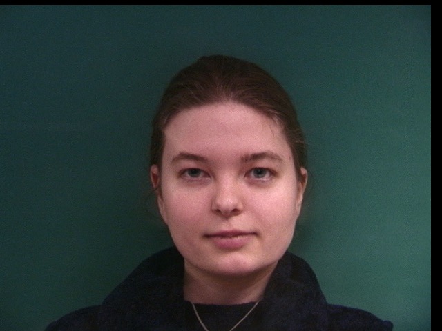
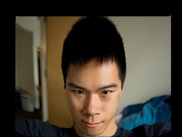
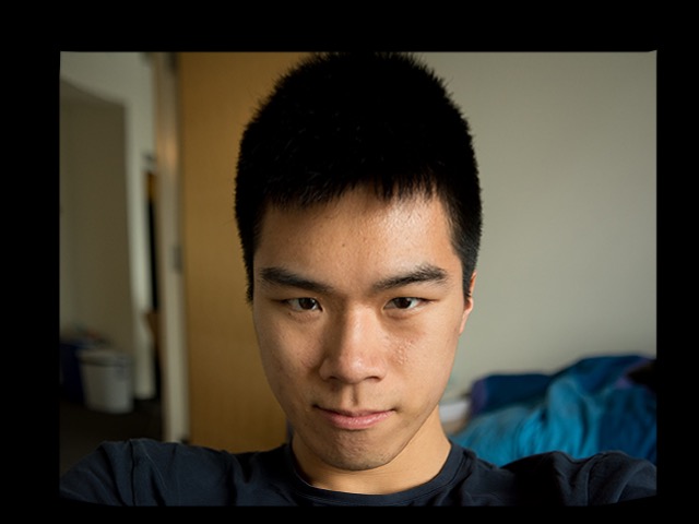
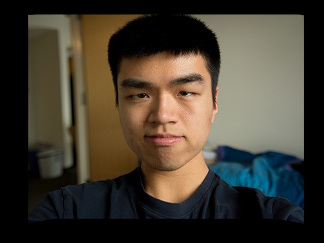
I labeled two images that had the same pose and lighting conditions. I computed the average of their keypoints matrix, and then I ran an algorithm for Delaunay triangulation on this average. I warped the two images into their halfway point, by using the average keypoints matrix and by giving each image’s pixels a weight of 0.5.


The result looks very convincing, except for the glasses and the ears. The glasses are a problem, because they appear 50% transparent in the final image, which is not a natural phenomenon. The ears also look bad, because Roger’s ears are hidden behind the hairline, while Vincent’s ears are in front of the hair line. So, there is an area where the algorithm tries to blend an ear with hair, which looks strange.
Other problem areas include the jackets and the exposed areas of the torso. The jacket was not annotated with keypoints, nor was the exposed area of the torso, so the algorithm makes no attempt to warp them in the final image.
Here is a YouTube video that shows the morphing process from the previous section. The first image displays for 30 frames. Then, the morphing is played for 45 frames. Finally, the second image displays for 60 frames.
The morphing is especially convincing in the teeth area, because both photos show roughly the same shape mouth and teeth arrangement. Although the jacket changes color dramatically, it is not as noticeable, because we tend to focus our attention on the face.
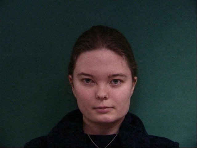
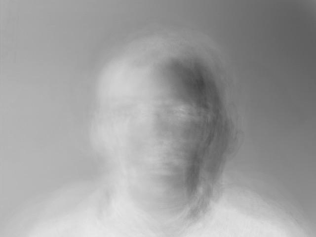
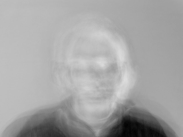
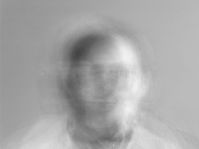
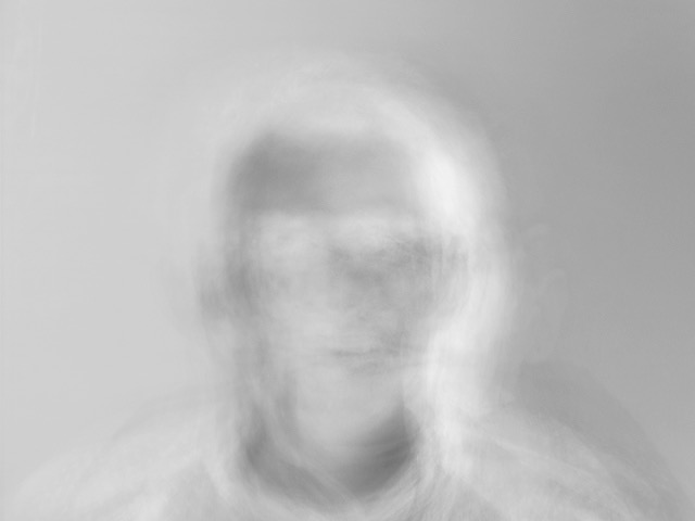
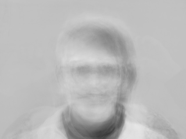
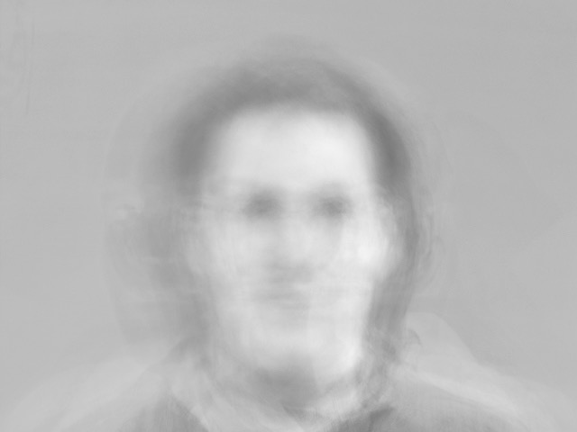
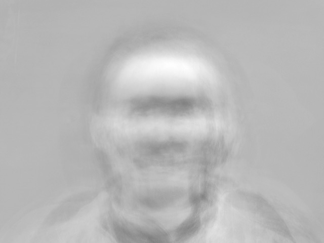
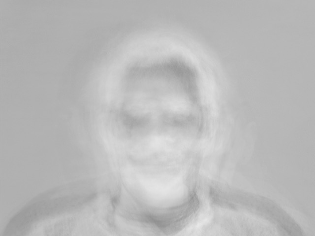
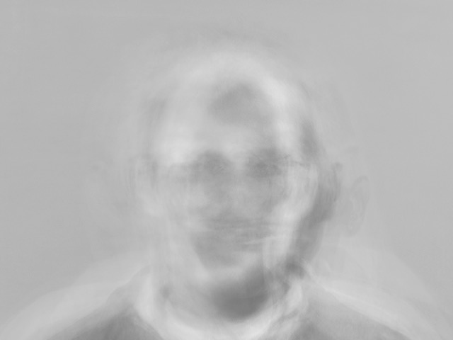
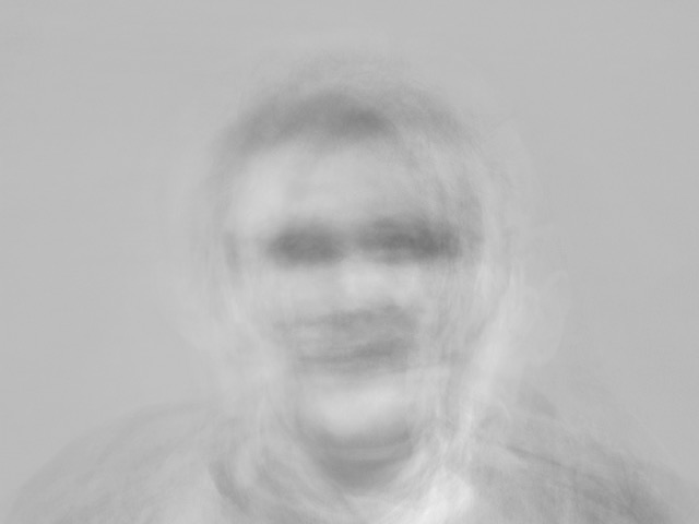
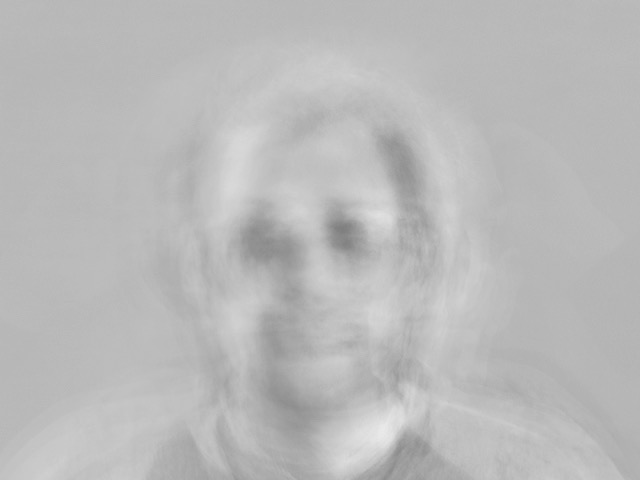
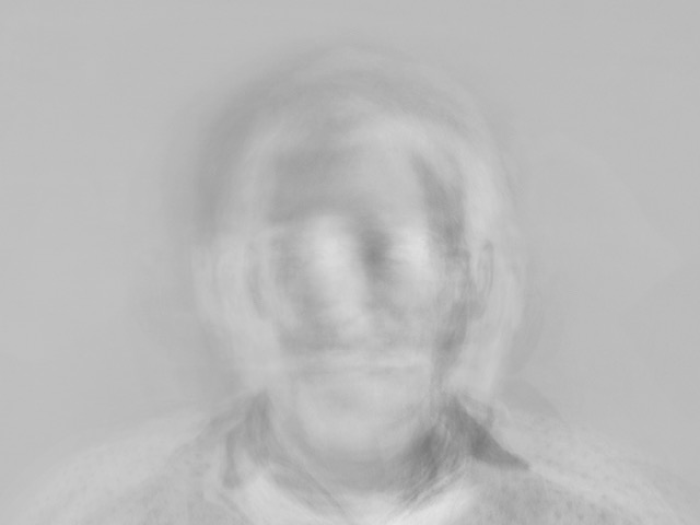
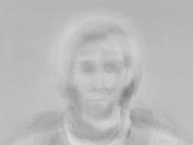
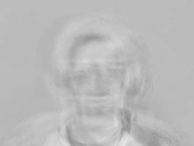
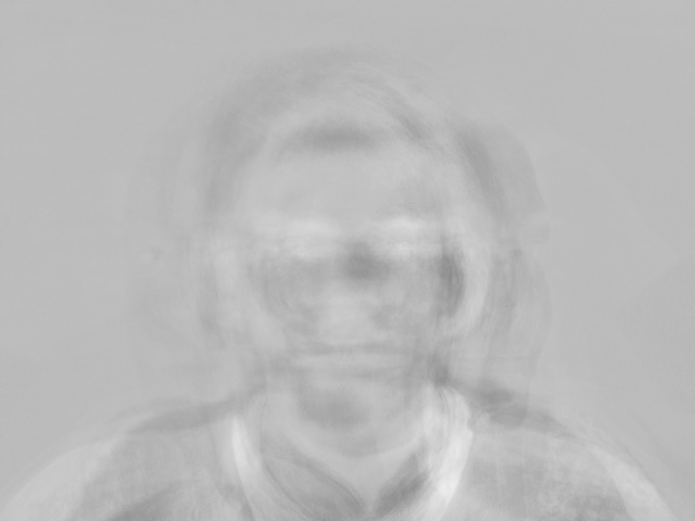
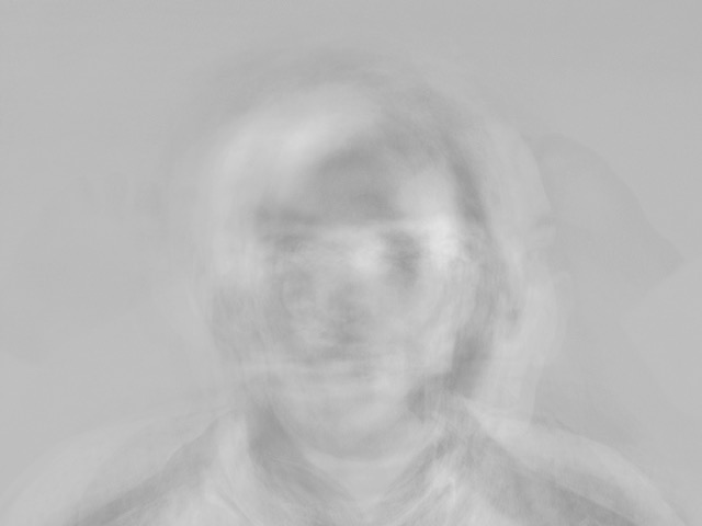
I downloaded this annotated face dataset of 40 faces with 6 poses each (240 images total). Each image is also annotated with the face’s gender. There are 33 male faces and 7 female faces. The average face is based off of the average keypoint geometry and the average face texture.
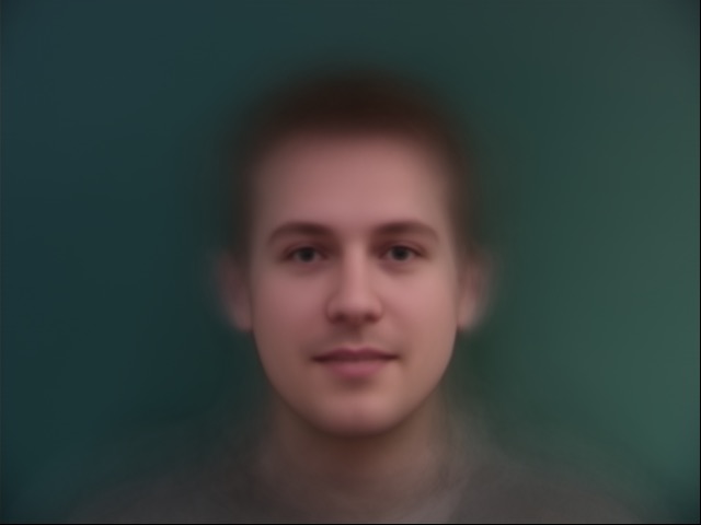
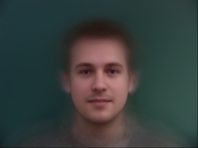
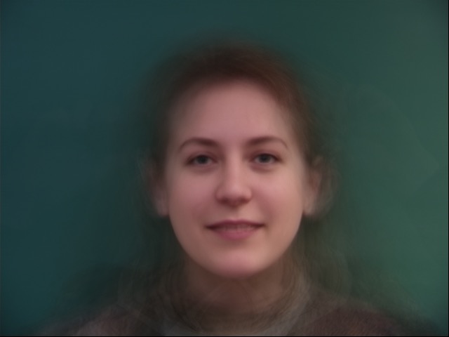
The average male face looks almost the same as the dataset average. This is probably because there are 33 male faces and only 7 female faces. The female face looks like it is smiling with teeth showing, whereas the male face looks like the mouth is closed. It might just be a coincidence that the females in this dataset smiled more in their pictures, and this effect would not be present with more data.
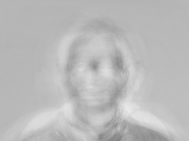
Now that I have the average of the faces in the dataset, I can morph each of the source faces into the average face. Here are two examples of this:
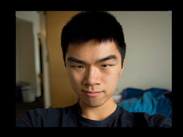
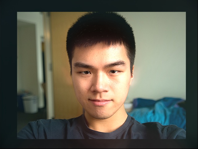
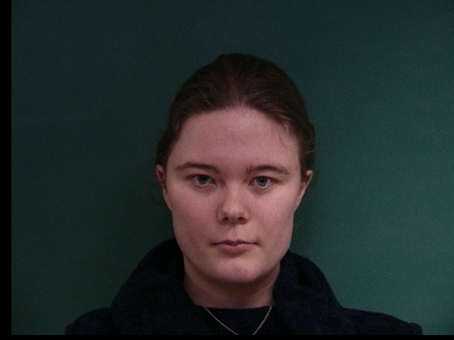
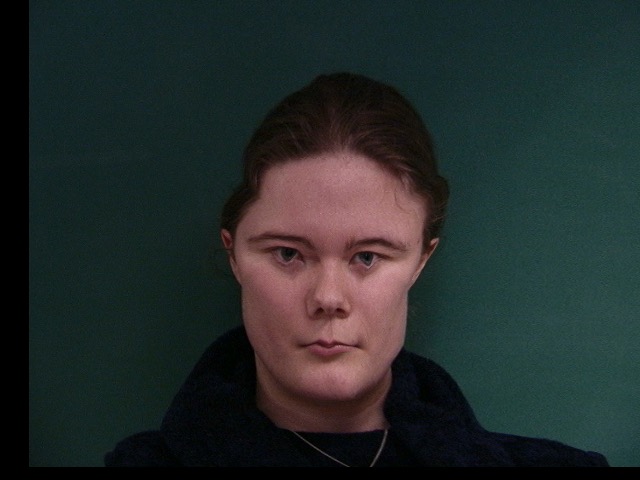
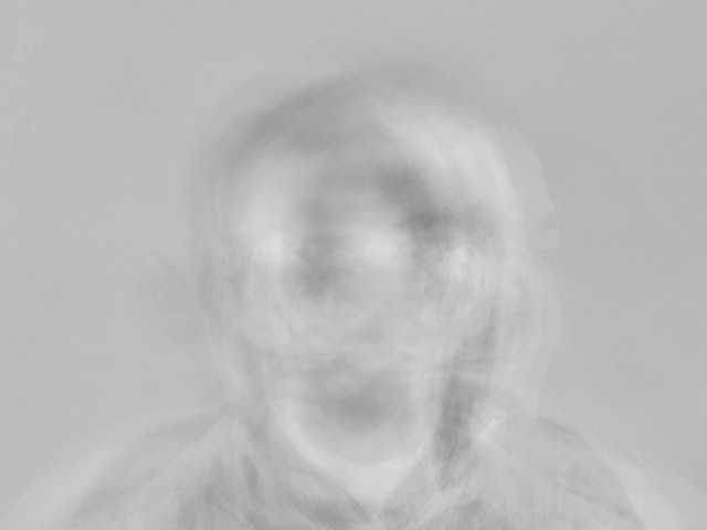
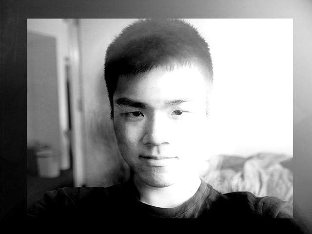
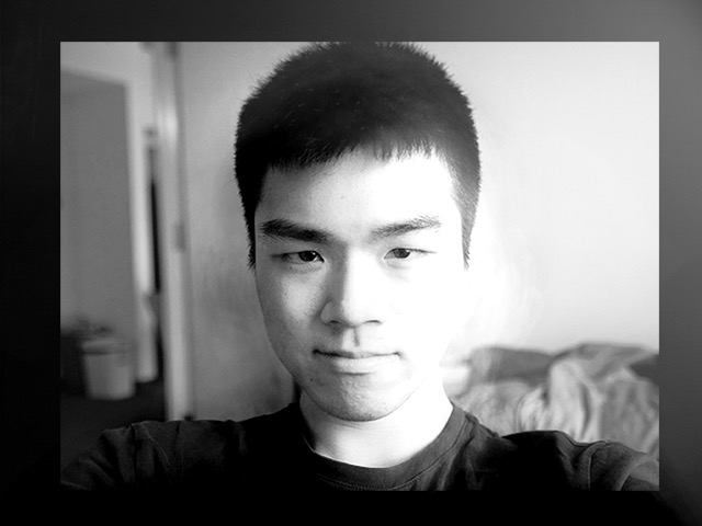
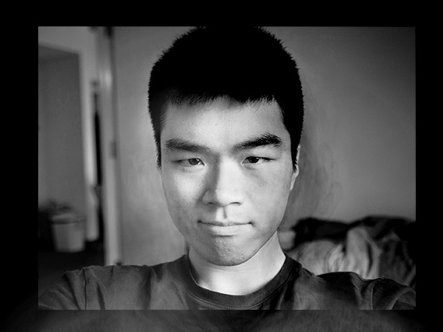
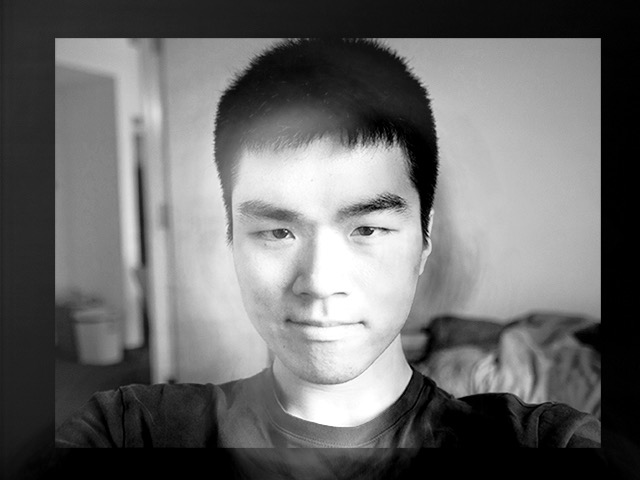
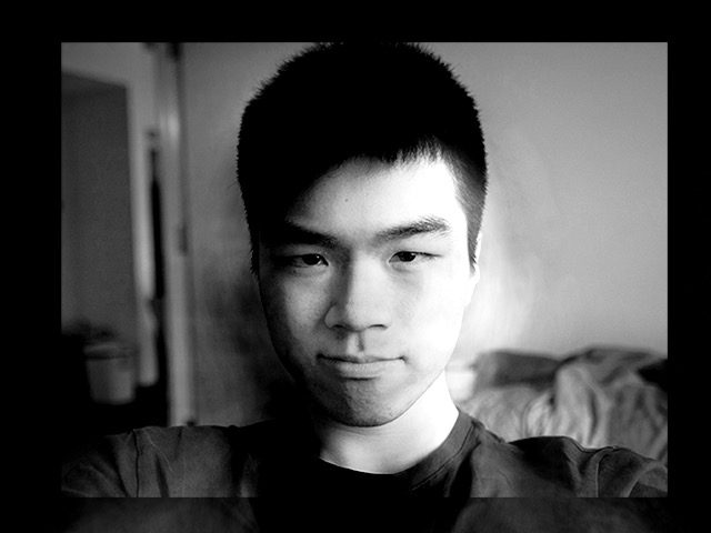
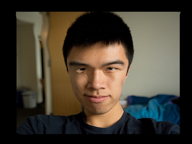
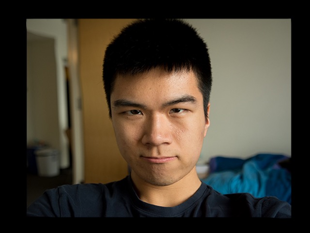
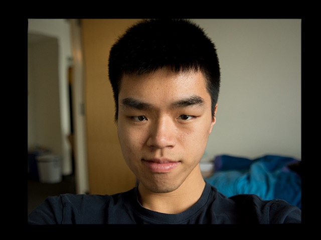
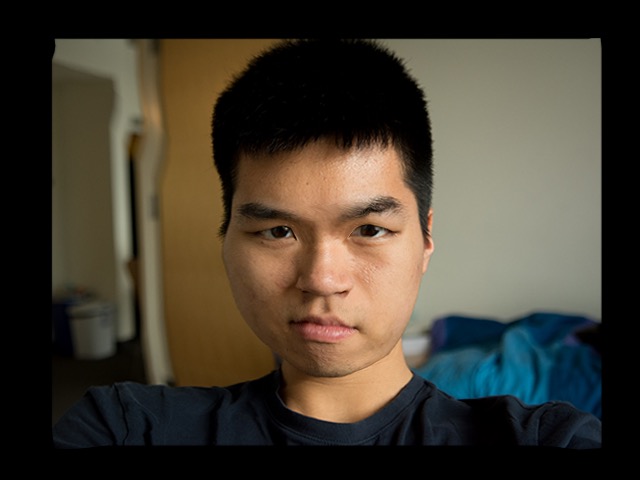
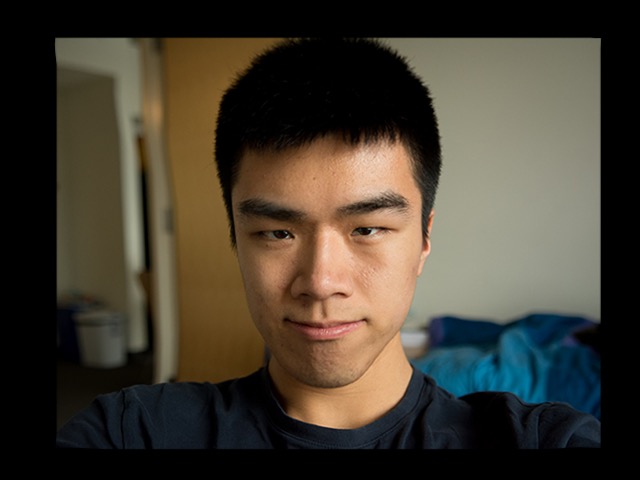
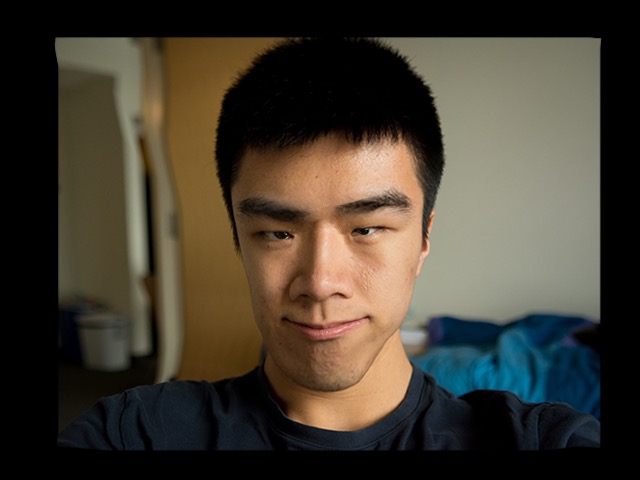
I also took a picture of myself and morphed it into the average geometry. Finally, I took the average face and morphed it into my geometry.

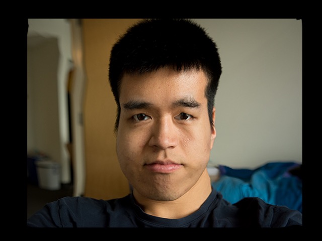
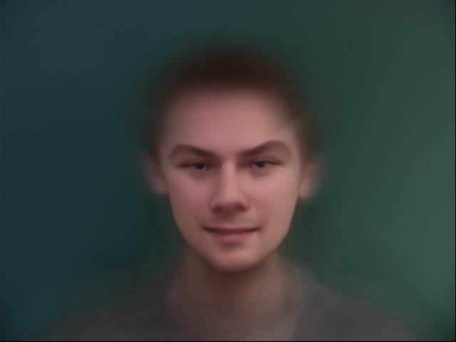
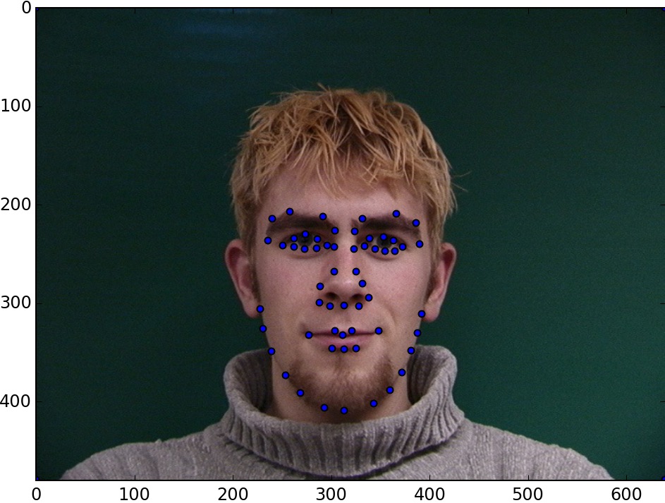
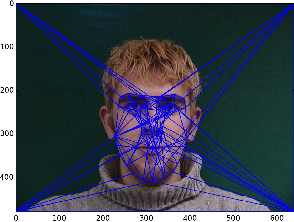
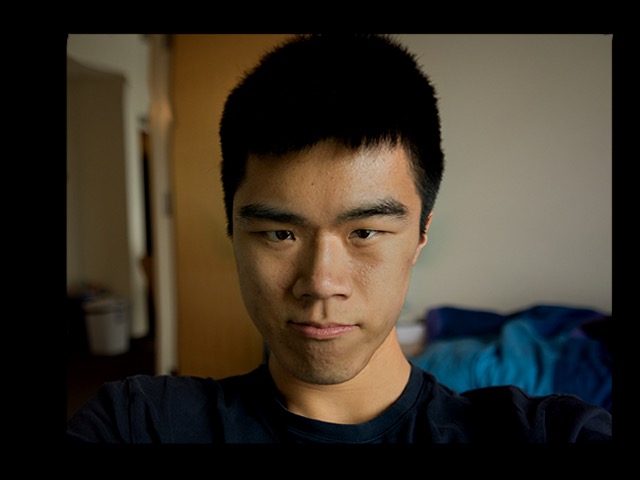
The results of this latest morph are very strange, especially because the keypoints in this dataset don't extend past the eyebrows. Take a look at this example of the annotated keypoints and the associated triangulation:
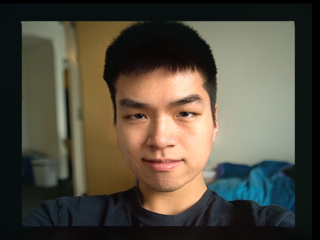
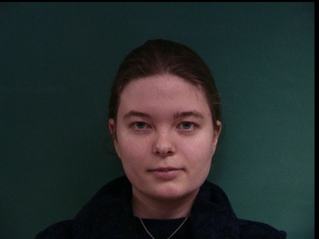
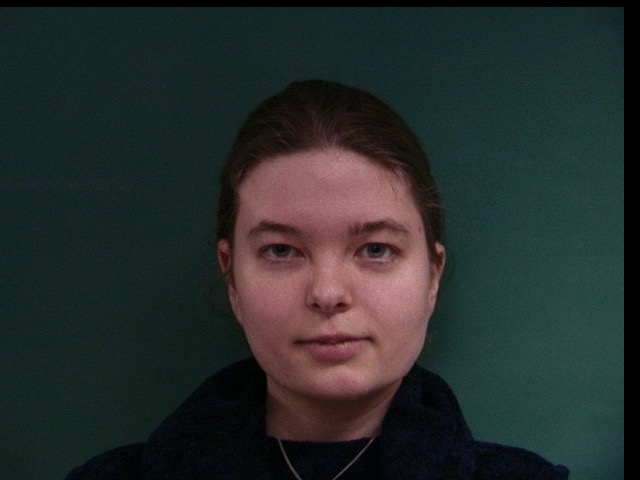
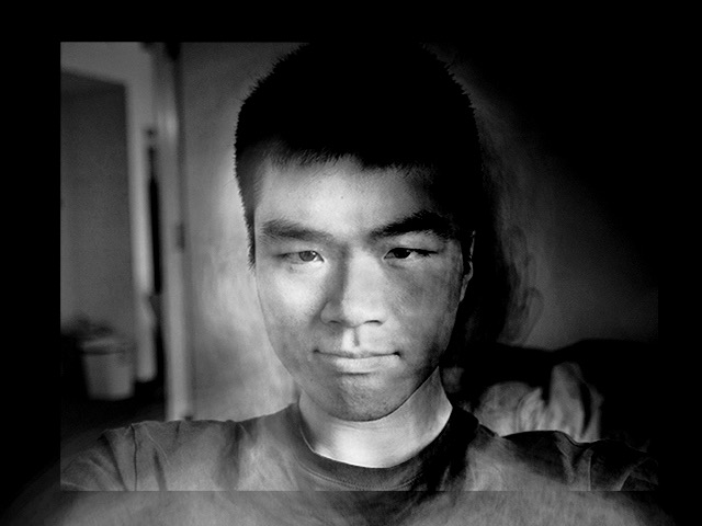
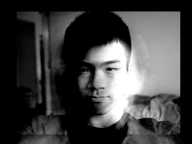
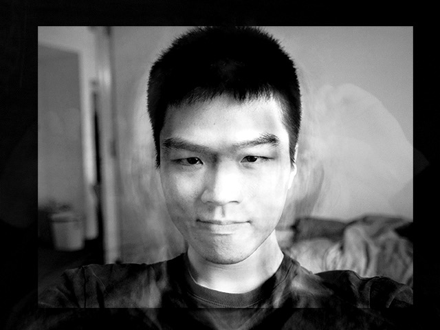
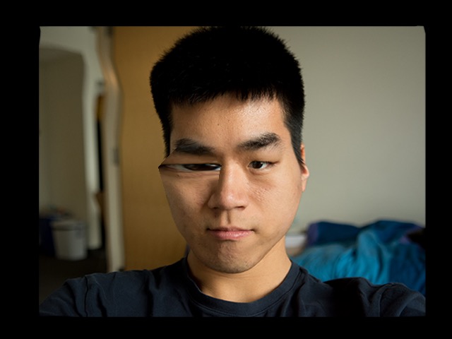
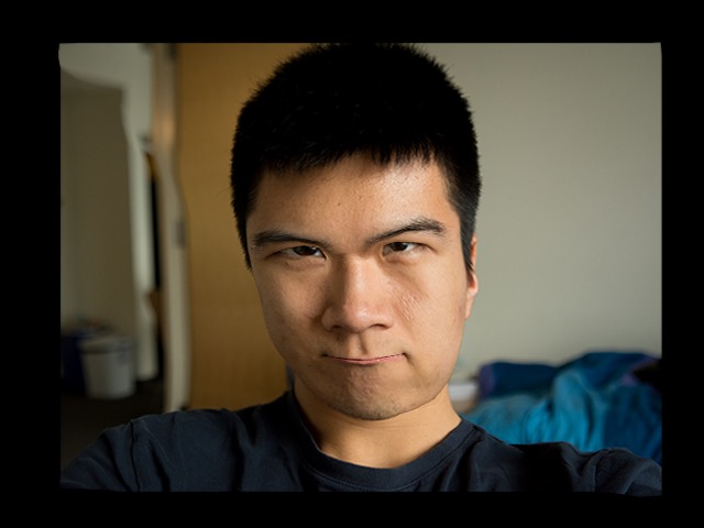
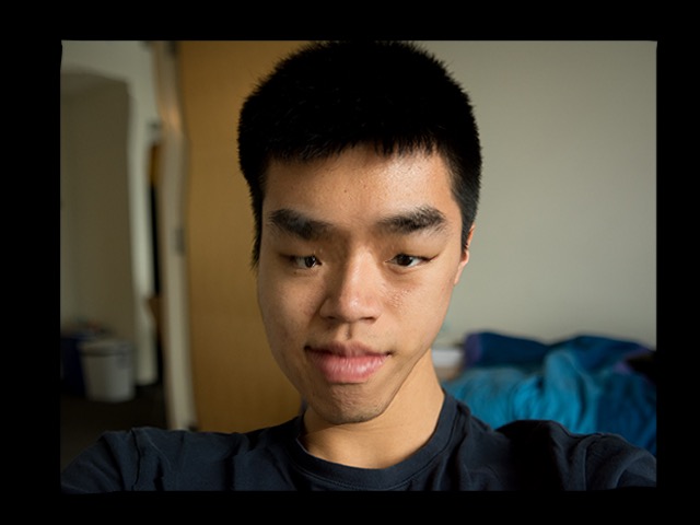
I used the annotated keypoints of my face and the average geometry of the dataset to extrapolate a caricature. The results are not very noticeable at a first glance, especially to people who are unfamiliar with the face. But, you can see that the eyes get thinner and the cheeks become thinner.
I also produced caricatures of 2 of the dataset images. I can’t see much of a difference between the original and the caricature. This is probably because I am unfamiliar with the faces. On the other hand, too much extrapolation would produce distorted images.
I took the difference between the female average geometry and the male average geometry to produce images that were morphed to be more female or more male.


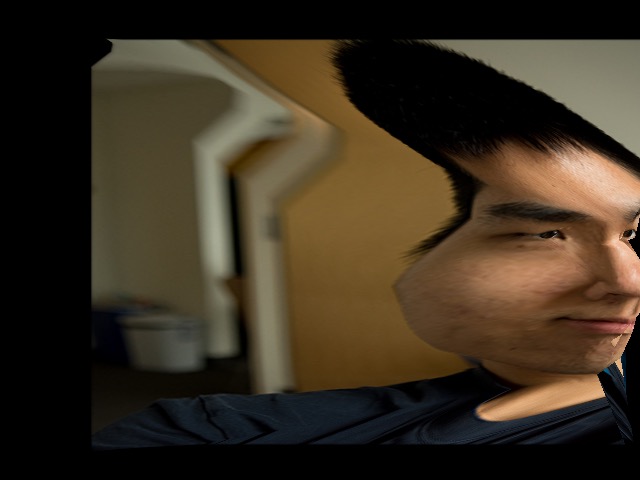
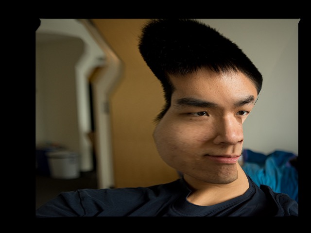
Pushing the face geometry toward the “male” direction makes the chin more pronounced and the face thinner. There is a lot of distortion in the forehead as the morph amount increases, which is probably caused by the lack of annotated points above the eyebrows (as well as a slight misalignment of the dataset faces that are male vs female).
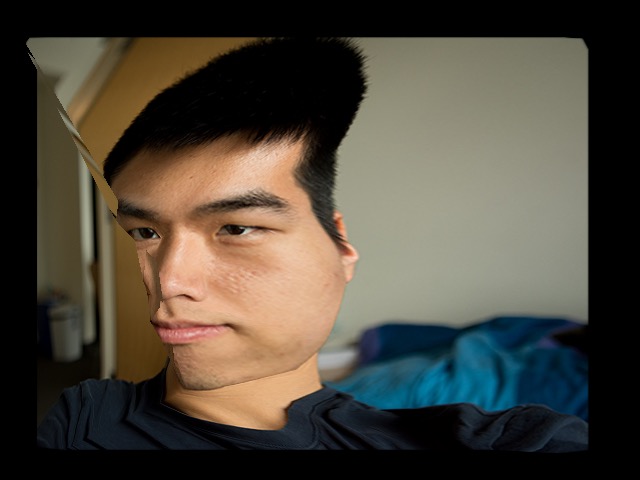
The same can be done in the opposite direction to get more feminine geometry.
I also tried using the difference in the face textures of the males versus the females, but the effect is not as convincing.
Finally, I can apply both techniques together to see their combined result.
I also tried this technique on some of the faces in the dataset. Here is an example of using this technique on a female face:
The dataset can be expressed as a 240×480×640×3 matrix. If I flatten the 2nd, 3rd, and 4th dimensions, then I can use the usual PCA techniques on the resulting data matrix. Actually, I first converted the RGB images to HSV, and extracted just the value component, so my dataset became a 240×480×640 matrix. Then, I flattened it to 240×307200 matrix. I did this because the colors didn’t make sense after processing (and made it harder to visualize negative values), and also because it saves some memory.
The same analysis can be applied to the keypoint matrices. The annotated keypoint data can be expressed as a 240×62×2 matrix (there are 58 keypoints, 4 corners, and 2 dimensions — x, y). I flattened this to a 240×124 matrix.
I was interested in finding what the principle eigenvectors was, but it would take too much memory to store the covariance matrix of the design matrix (which has a size 307200×307200). So, I used the compact PCA trick and first computed the eigenvectors of the 240×240 matrix and then multiplied the design matrix against them. The first 20 eigenvectors are visualized below.
I applied some of these eigenvectors to the image of my face (which is now in grayscale, because I took only the value component). This helps to visualize the purpose of each eigenvector.
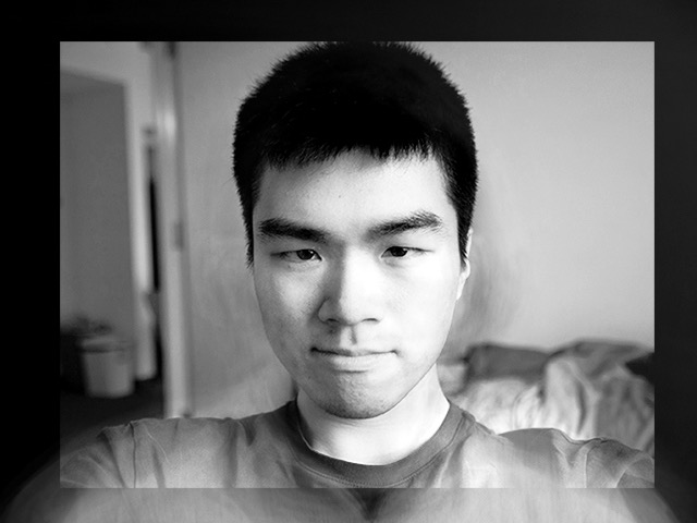
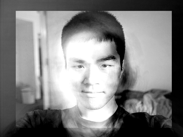
The first eigenvector seems to be responsible for the left-right lighting conditions of the image. This is reasonable, since some of the faces in the dataset were photographed with a flash from camera-right.
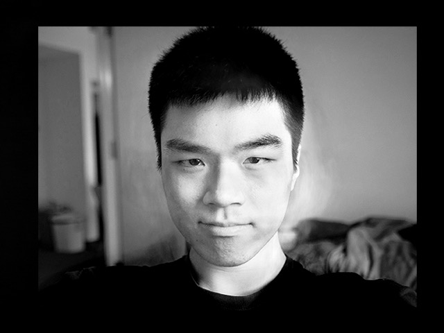
The second eigenvector seems to be responsible for the lightness or darkness of the clothing.
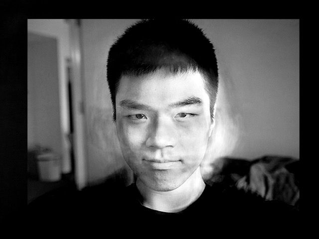
The third eigenvector corresponds to slight variations in the head position.
I noticed in some of the low-energy eigenvectors had a very distinct hand shape on the left and right side of the image. I searched through all the faces in the dataset until I found the image that was causing these to appear. It seems like a single odd image can influence the PCA of a dataset that contains 240 input images. The hand is noticeable in eigenvectors as high as 5th eigenvector.
I took the 240×62×2 data matrix of keypoints and ran the usual PCA technique on it. The eigenvectors of this matrix are hard to visualize by themselves, so I just applied them to the geometry of some of the input images. The result of the modified geometry should reveal the nature of these eigenvectors.
Here are the three principle eigenvectors of the keypoints matrix. They correspond to the left-right displacement of the face, the up-down displacement of the face, and the size of the face. These are all pretty reasonable.
The 10th eigenvector seems to correspond to the width of the right eye. (See below)


The 11th eigenvector has something to do with lip size, but also the position of the eyebrows.
The 18th eigenvector seems to be a good approximation of square chin vs rounded chin. This can make a face look more masculine or feminine, and actually seems to be more convincing than the gender modification code in Part 6.

Altogether, these geometry eigenvectors can parameterize a person’s face by describing things such as the position and proportions of their facial features.
Faces are a great data source for image processing techniques. Almost all faces blend smoothly into other faces, except for the presence of special features: glasses and hair (facial hair and hairline). However, the techniques do not work as well when the keypoints are not sufficient to completely label the important parts of the image. The dataset I used did not have keypoints above the eyebrows, so there was a lot of strange effects in the forehead area.