Roger Chen
In this project, we used compute homographies using a set of labeled feature points in a pair of images. Then, we use multiresolution blending to create a composite of many images, which results in a panorama image.
I used my DSLR and my cell phone camera to capture input images. I was able to set manual settings on both cameras, so that the exposure of the images would not change between shots.
I also created a point labeling web interface, which was used to label all of my image key points in these examples. The labeler supports adding, deleting, moving, loading, and saving arrays of points.
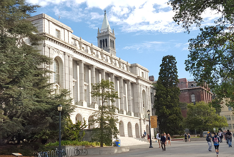
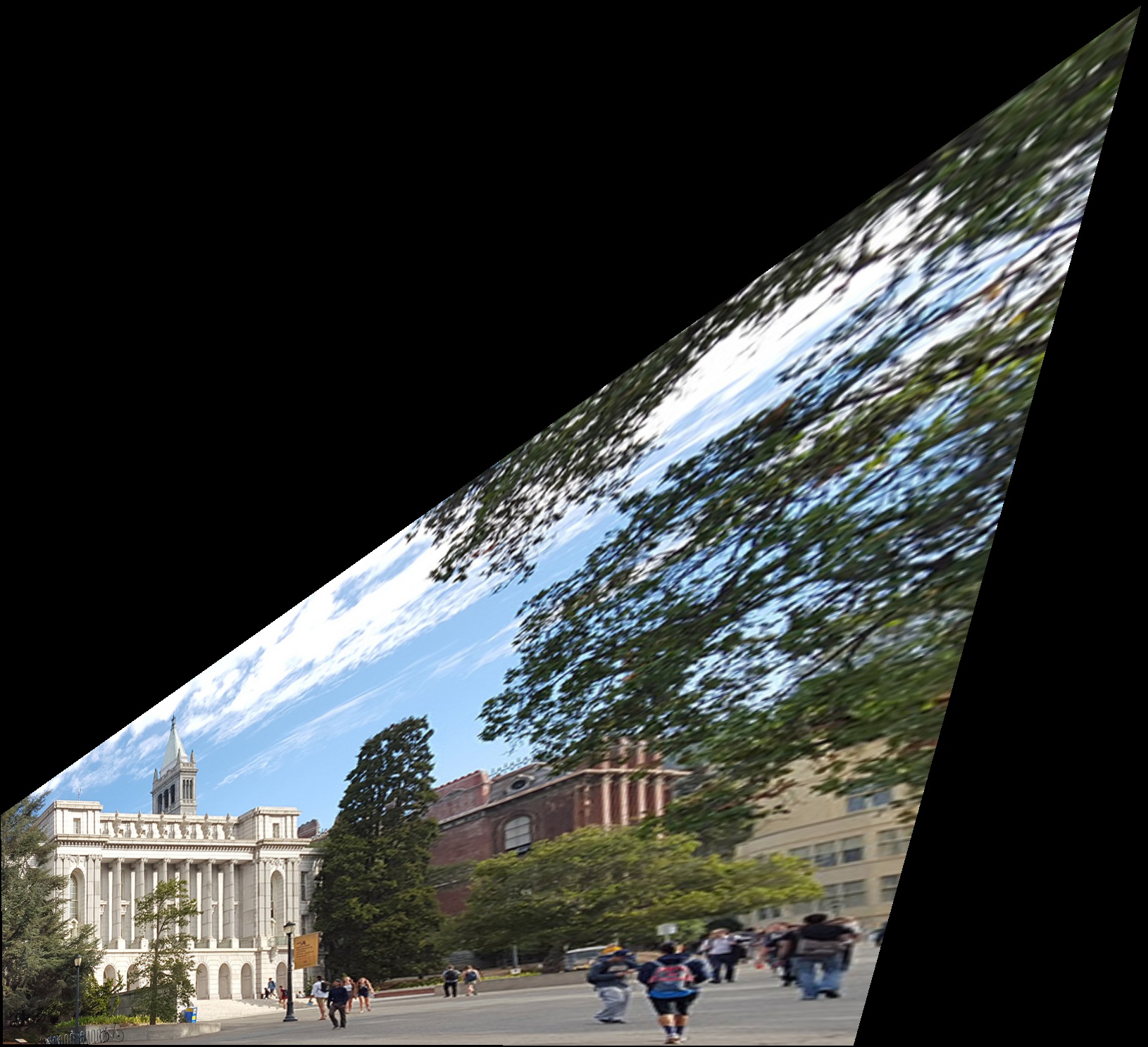
The first thing I did was to try some basic warping operations in order to test my computeH and warpImage functions. I took a picture of Wheeler Hall and warped it so that the face of the building was rectangular. This made the edge of the image very distorted, but I did get a good view of Wheeler Hall in the corner.
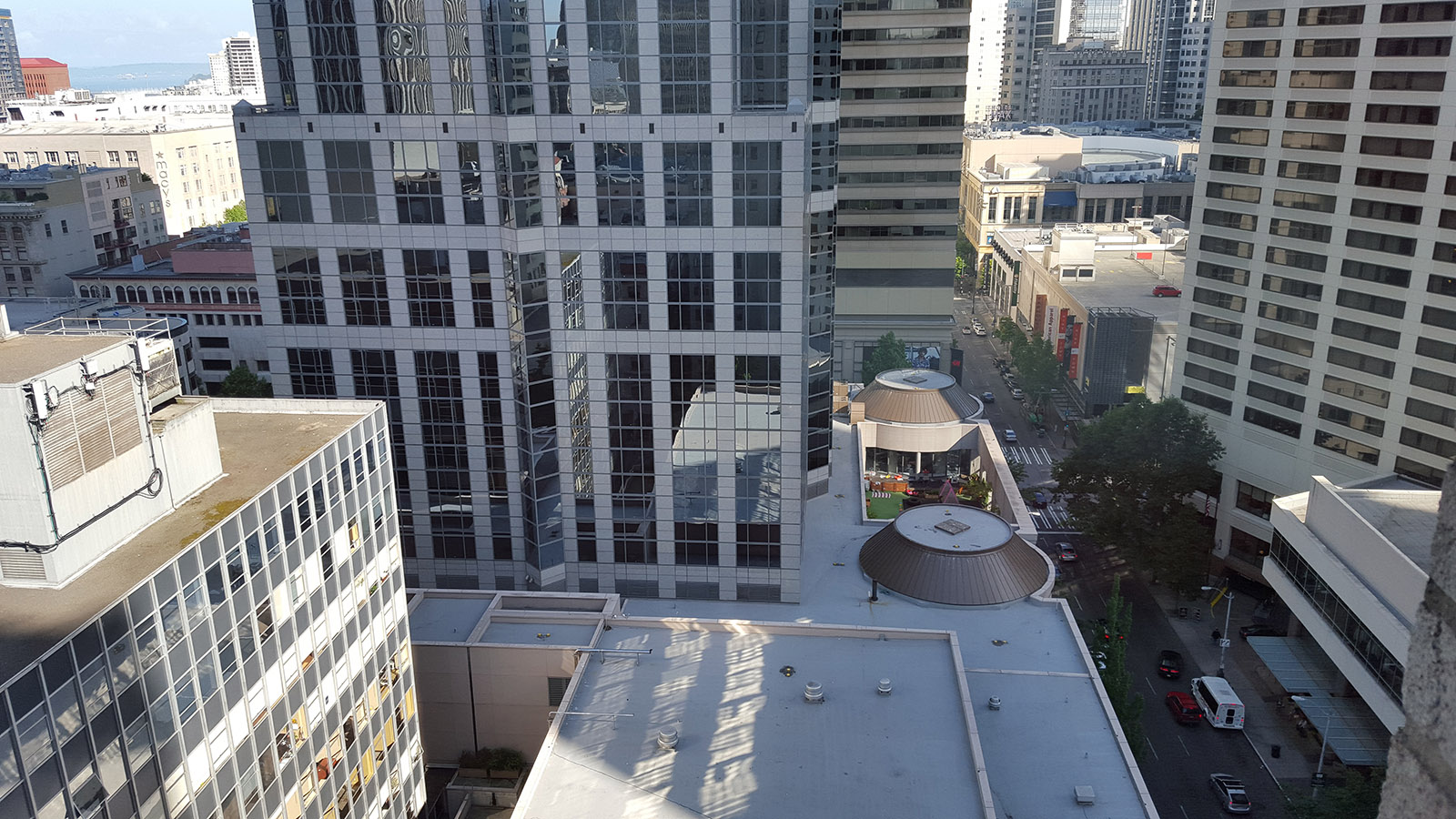
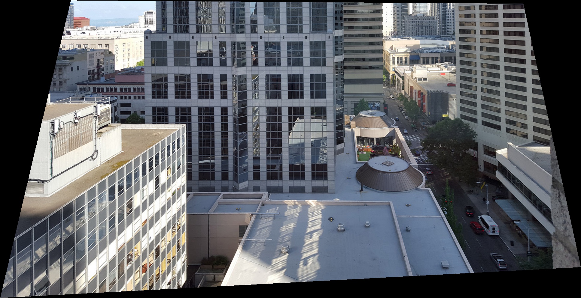
I tried the image rectification process on a different photo. This photo contains some buildings in Seattle, which were photographed from a high angle. I warped the image so that the large building in the center looks like it is rectangular.
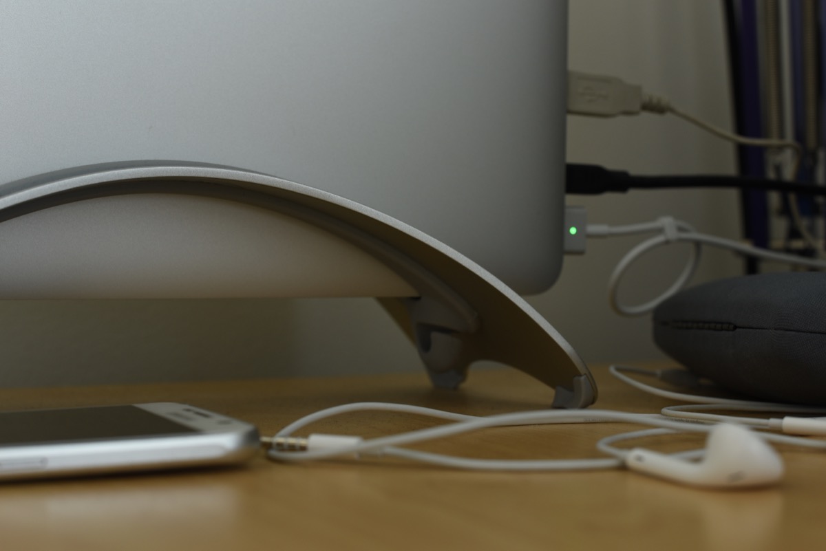
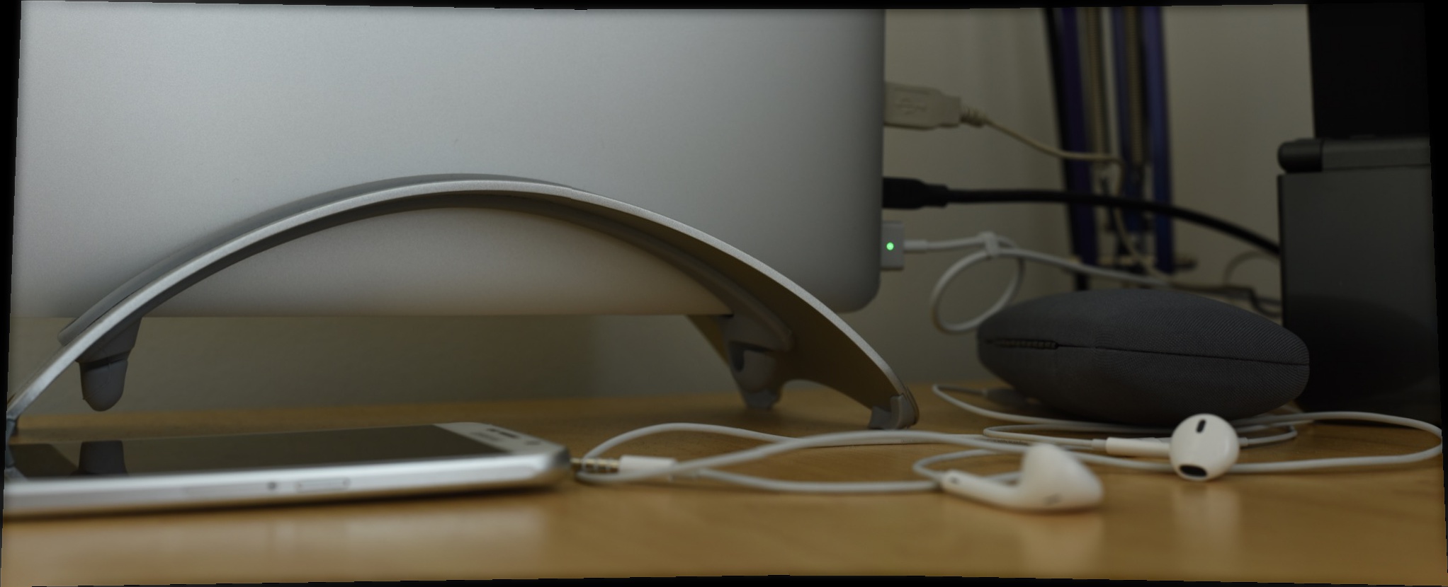
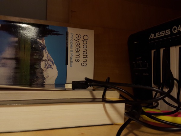
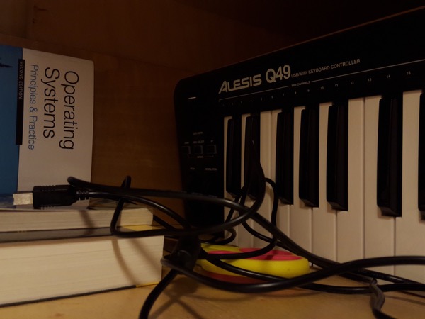
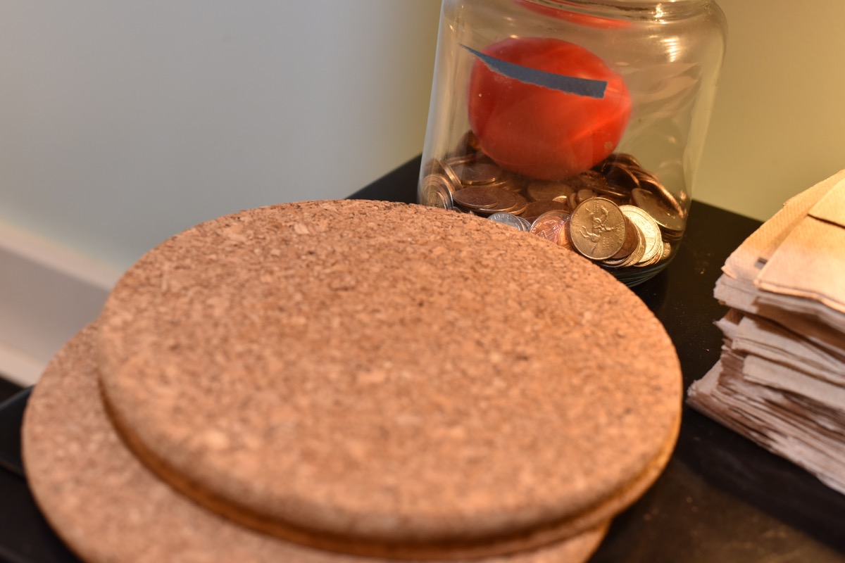
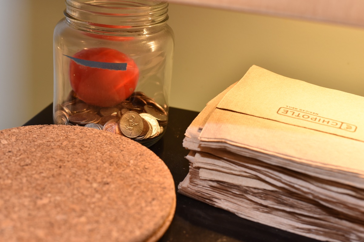
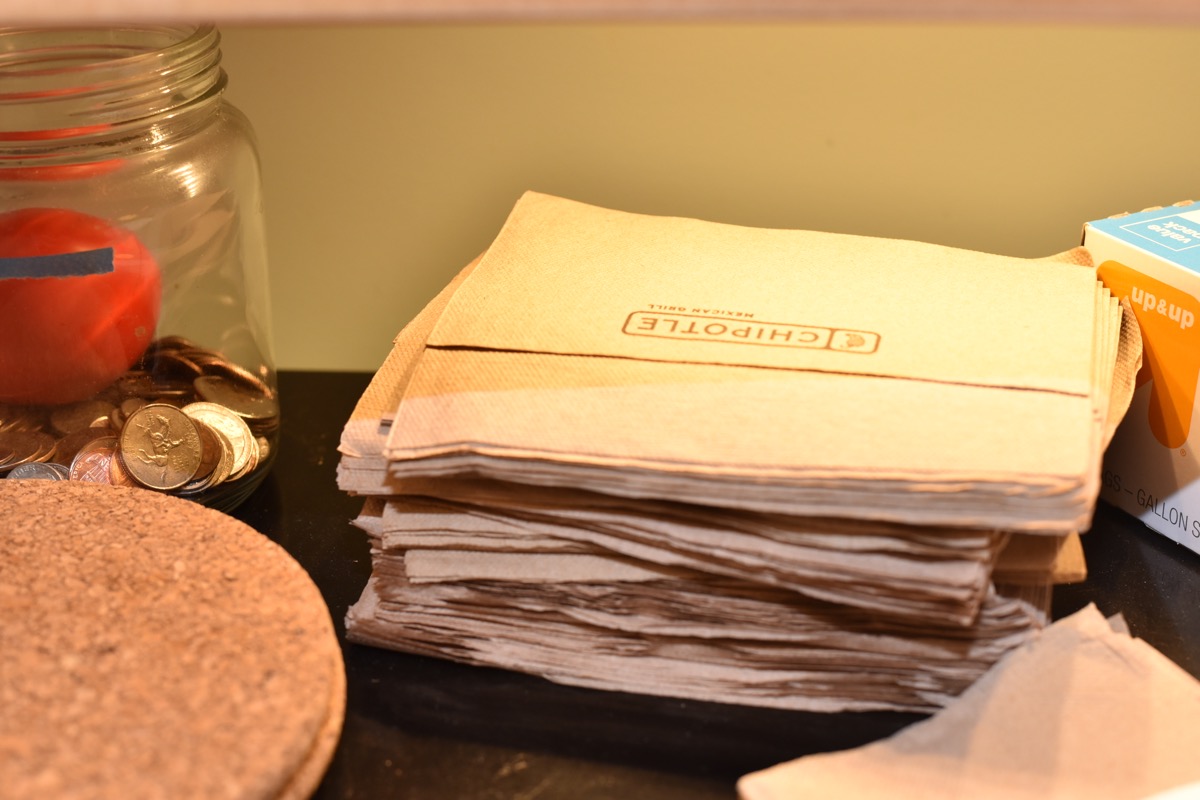
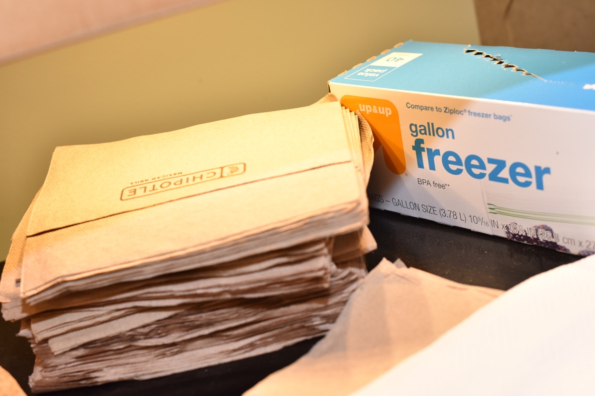
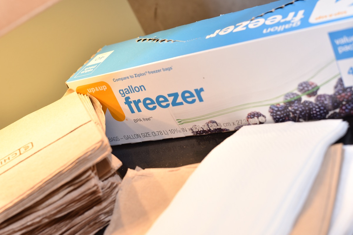
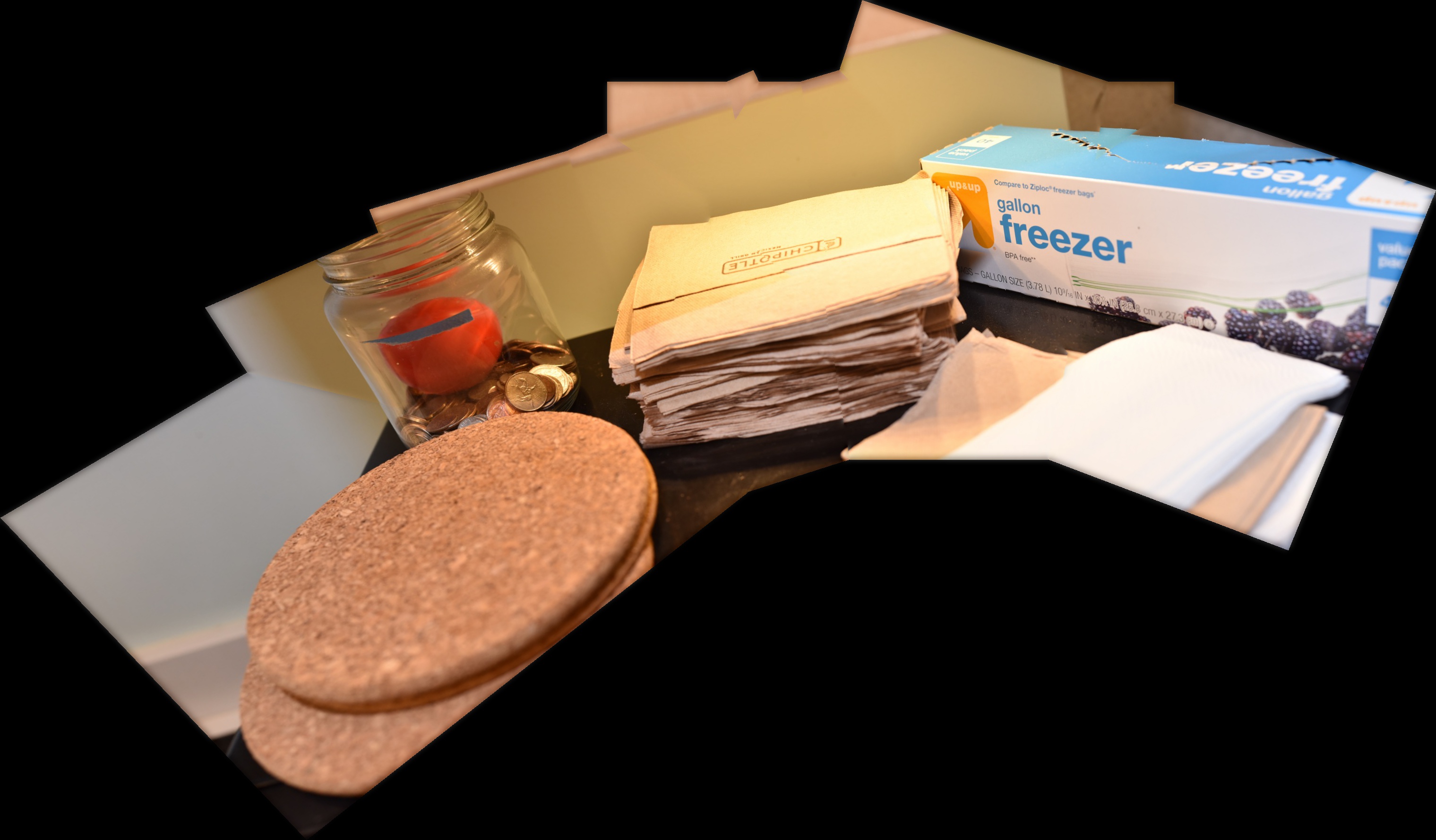
When I first wrote the program for blending multiple images together, I tested my code using a few pictures that I had taken of my desk, since it was the closest and most convenient location. However, the shallow depth of field of these photos made annotation difficult. There are not many sharp corners in these images to choose from.


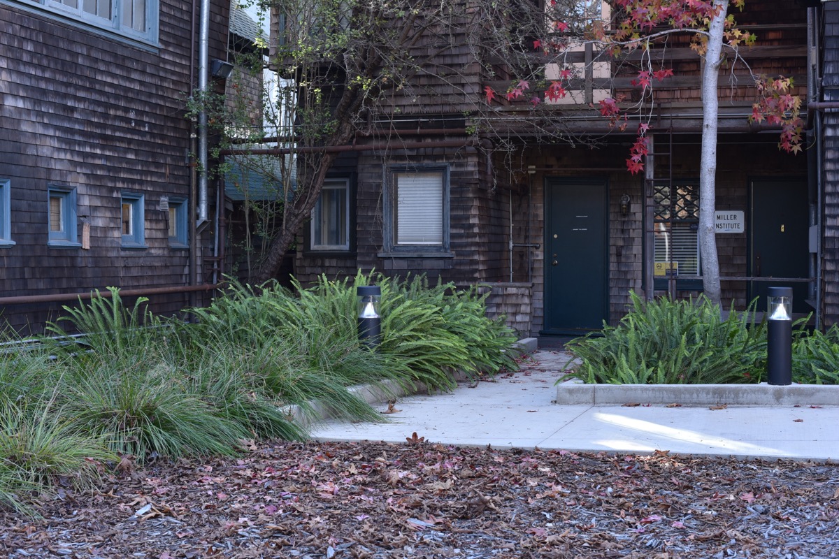
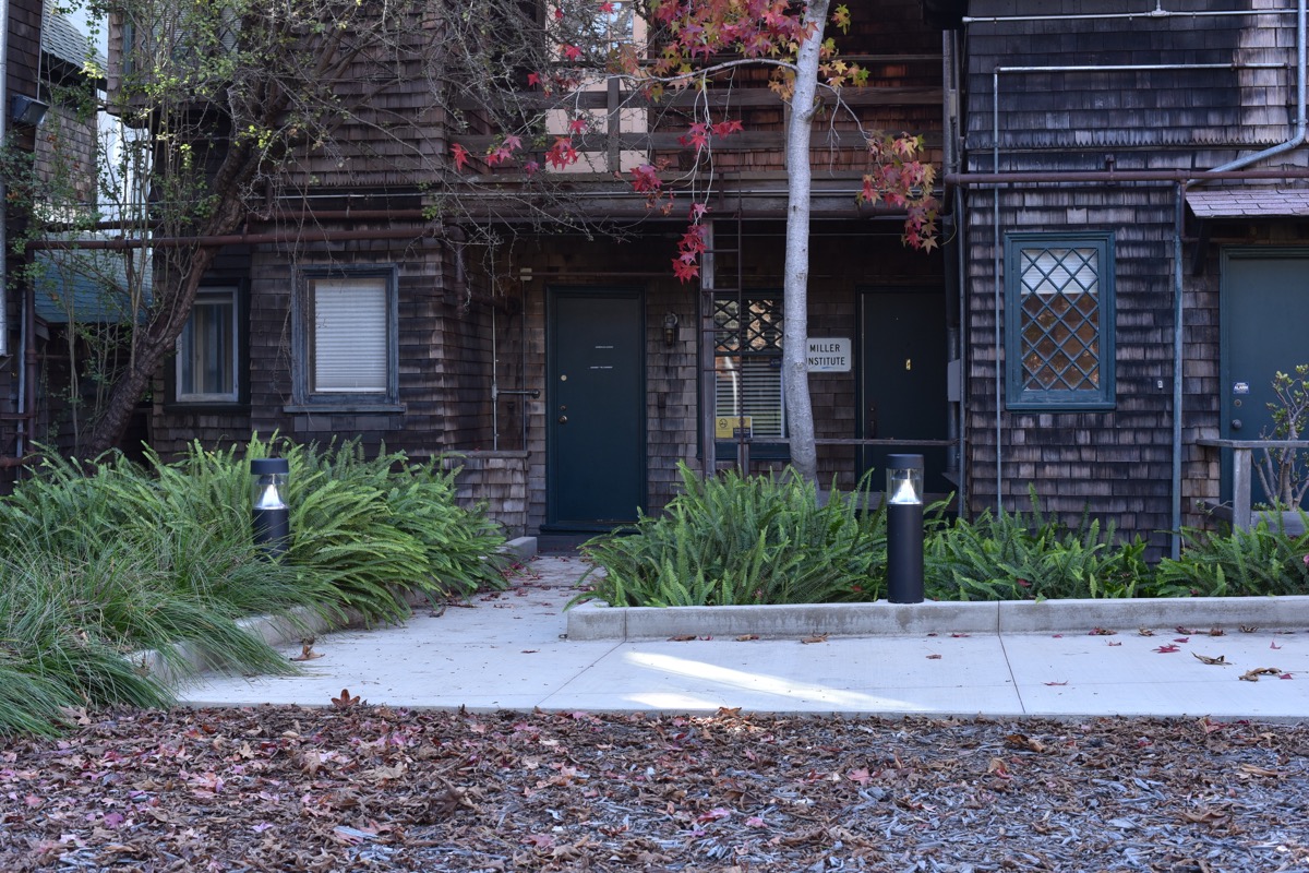
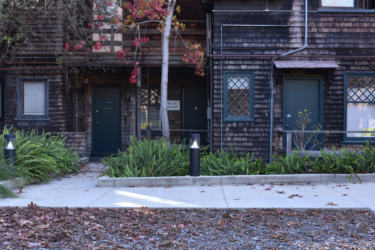
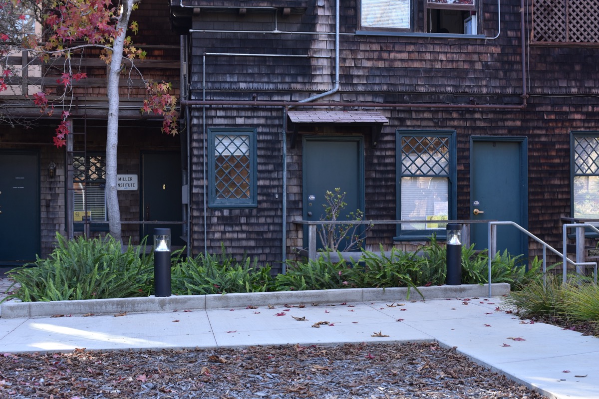
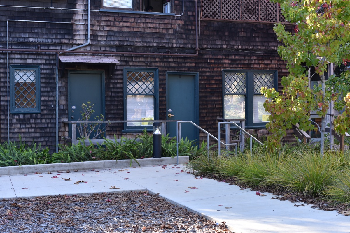
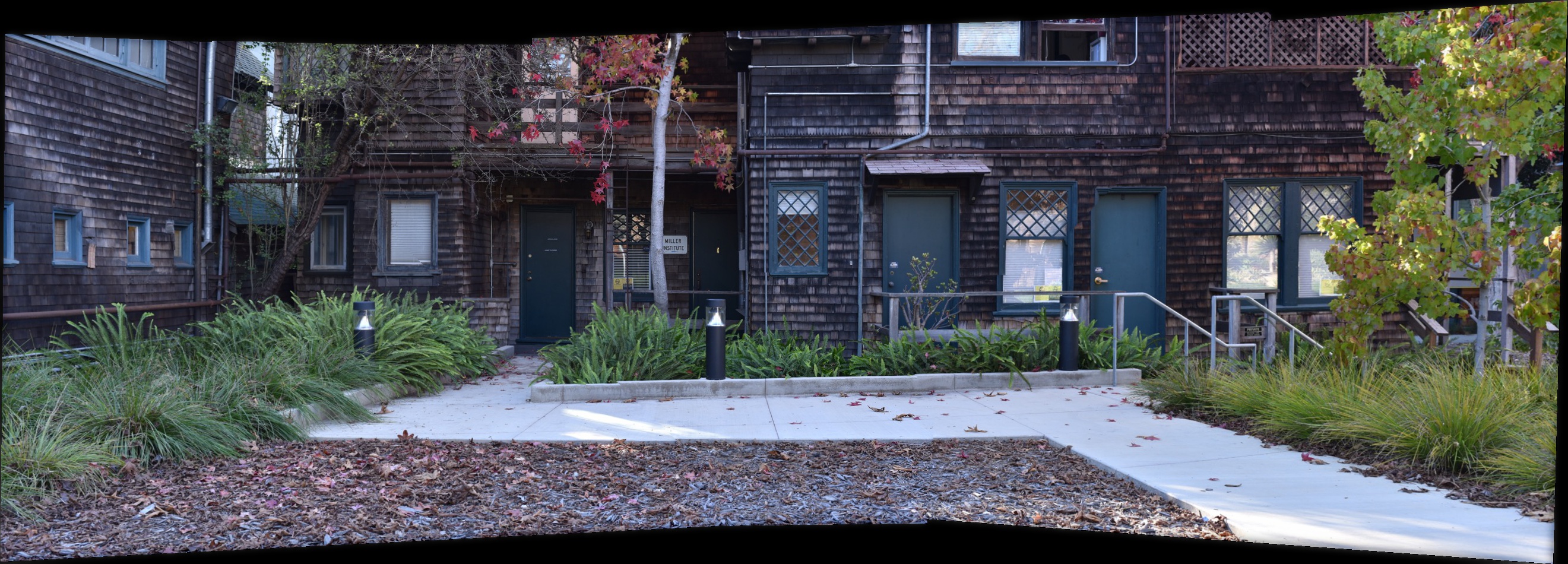
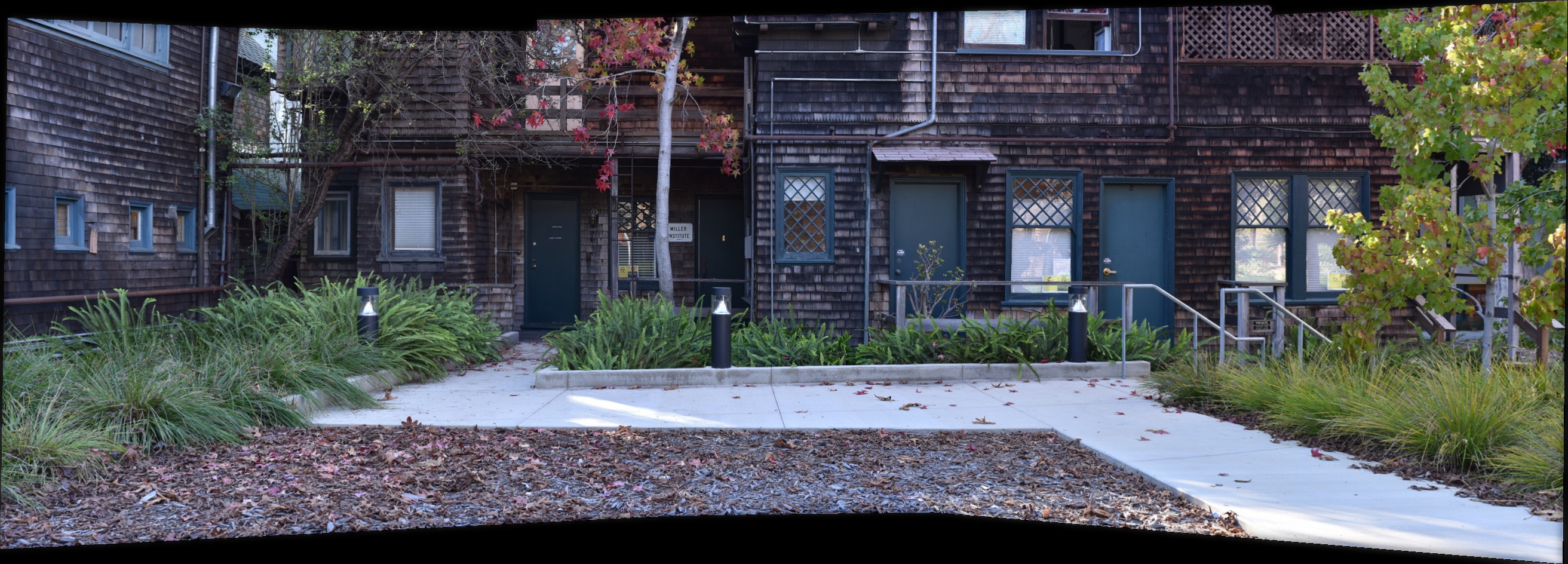
This set of images was easier to annotate, because there are a lot of fine details and textures throughout the scene.
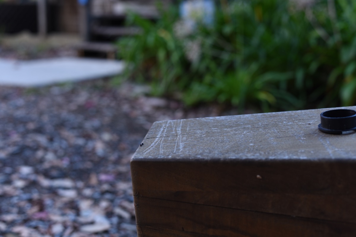
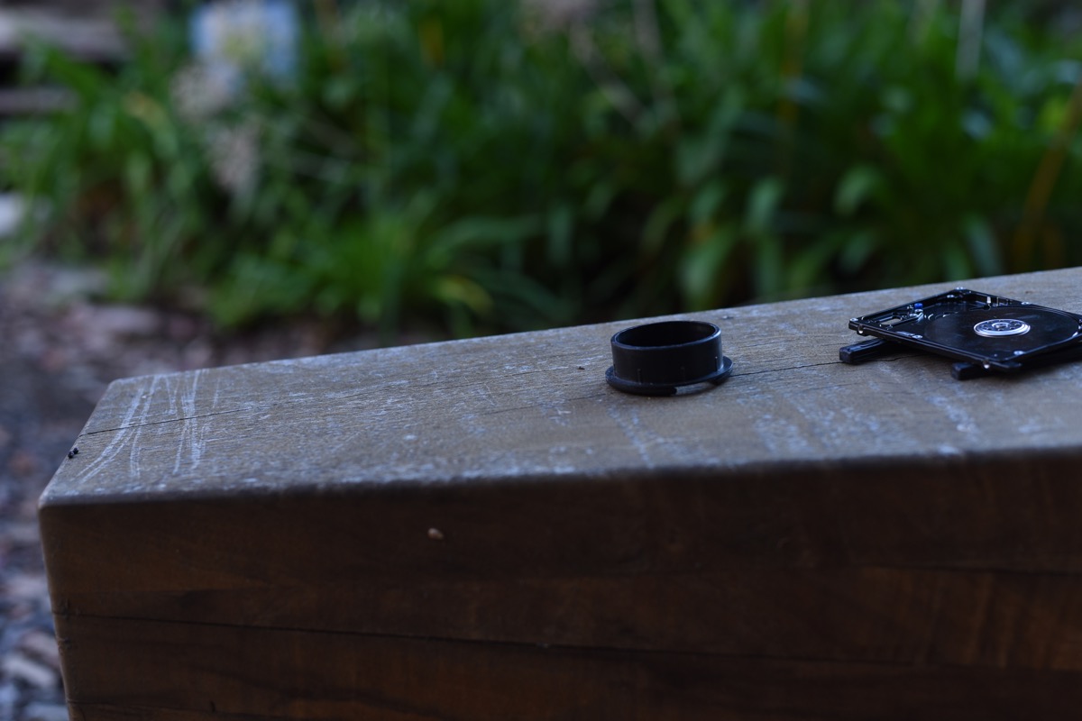
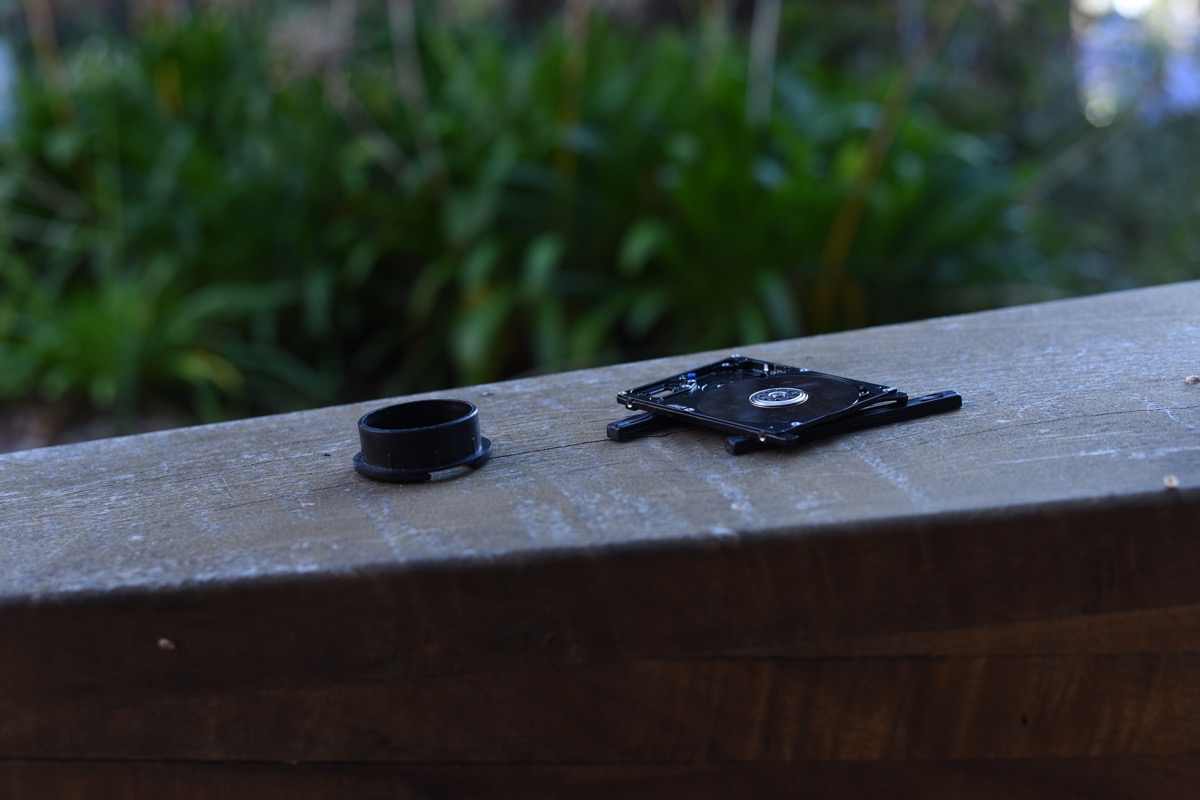
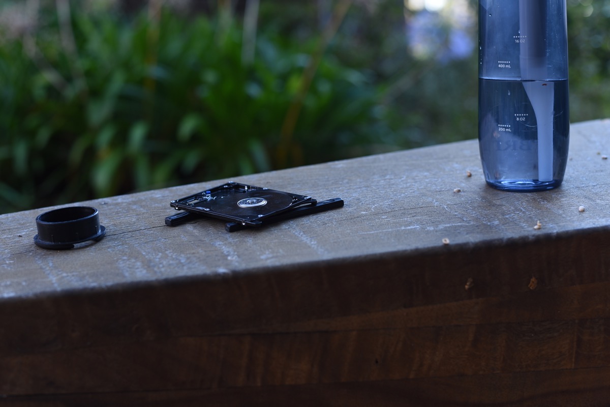
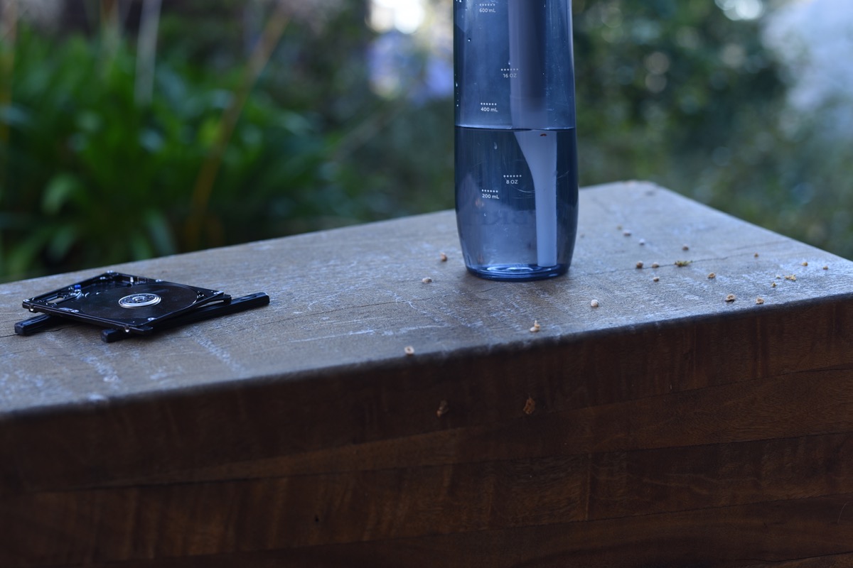
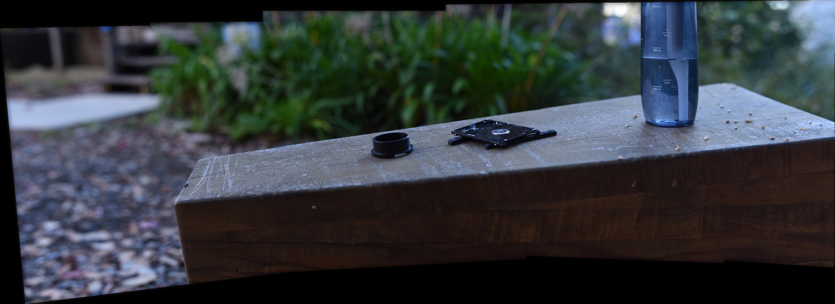
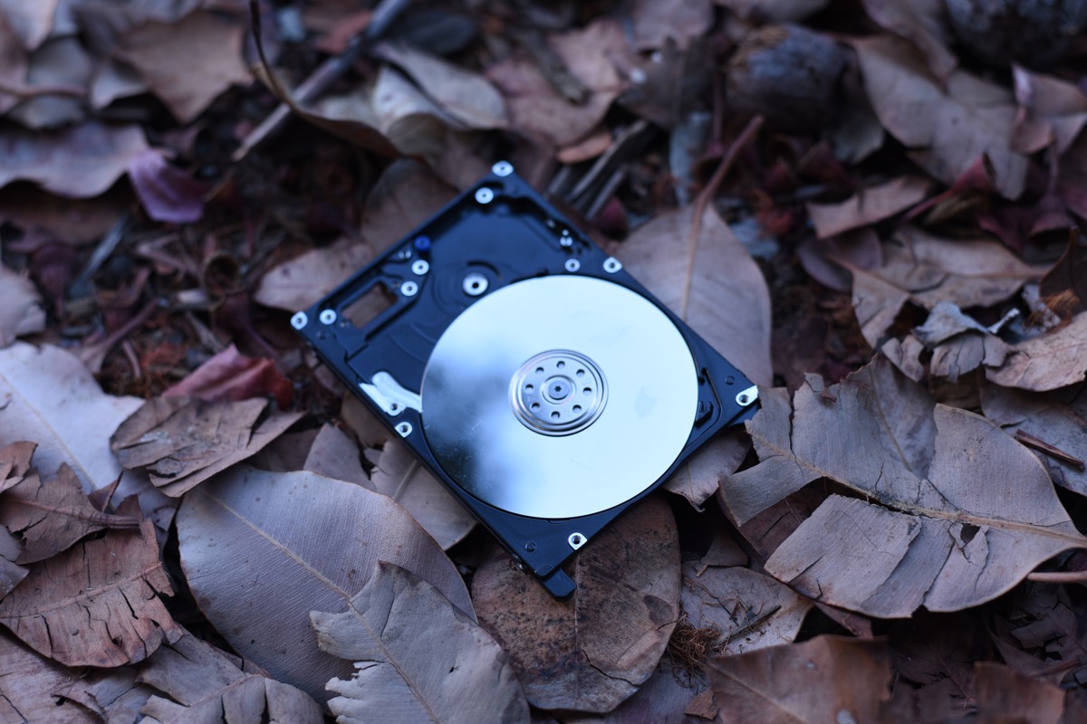
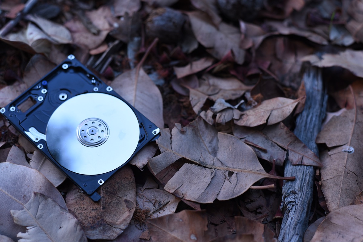
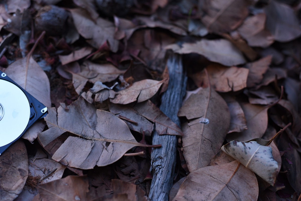
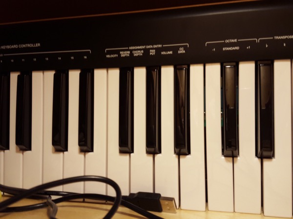
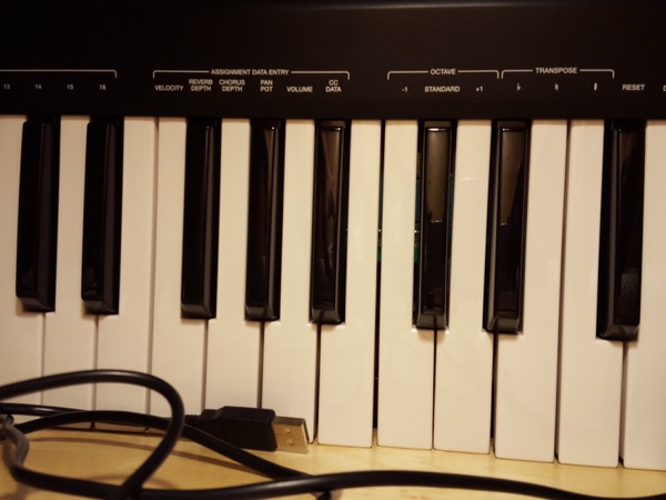
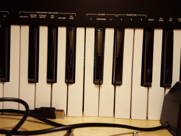
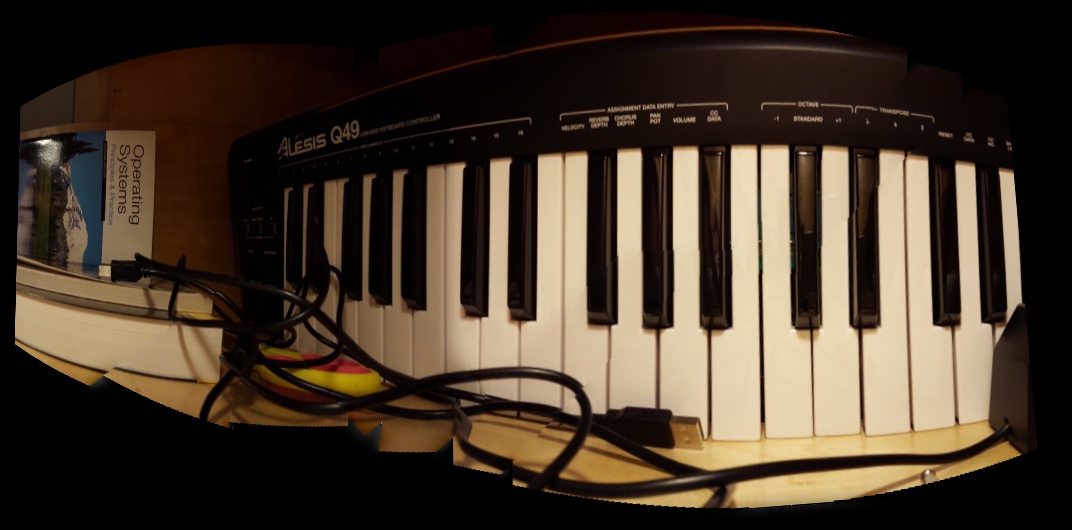
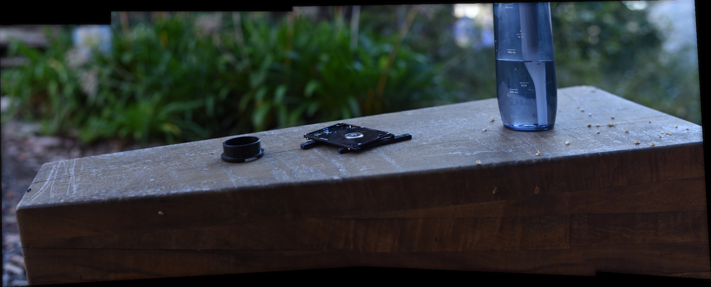
I took some more pictures of some of my belongings, including the cable organizer of my desk, my old broken hard drive, and my water bottle. The blurry background and flat wood texture made it hard to find points to annotate, but I was able to get a good mosaic with some persistence.
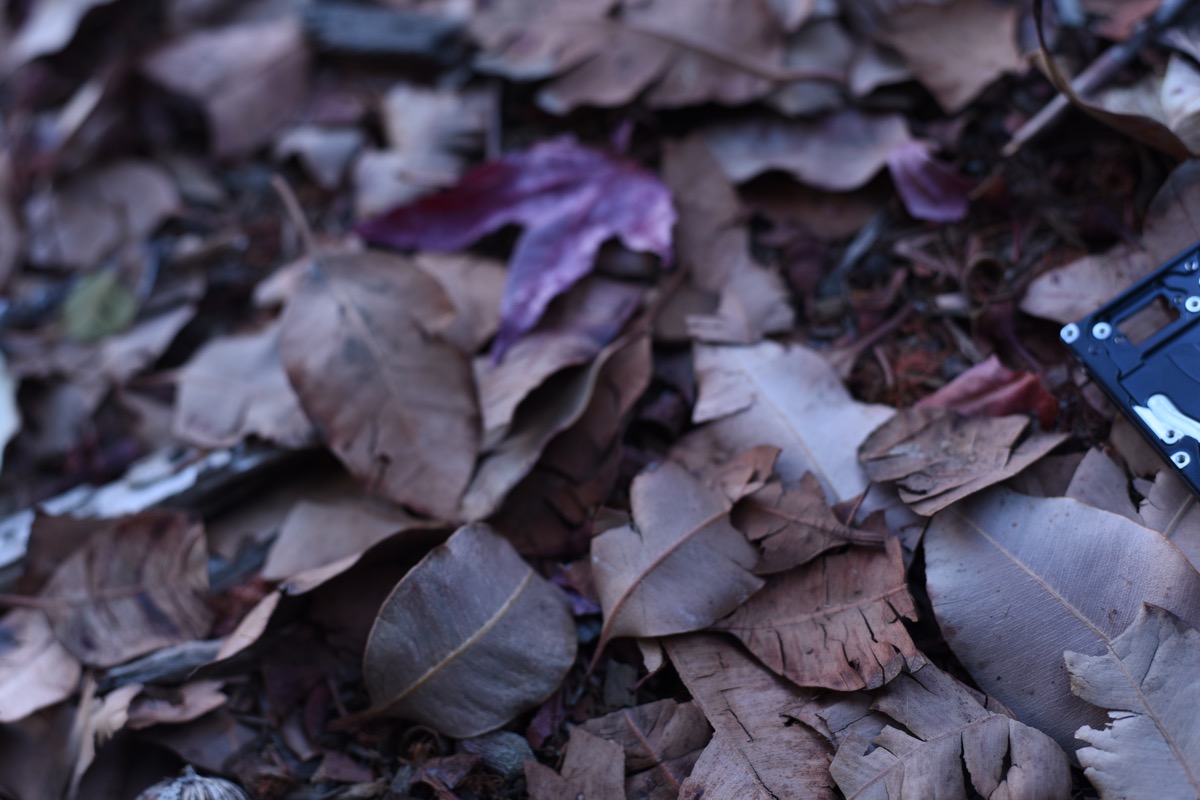
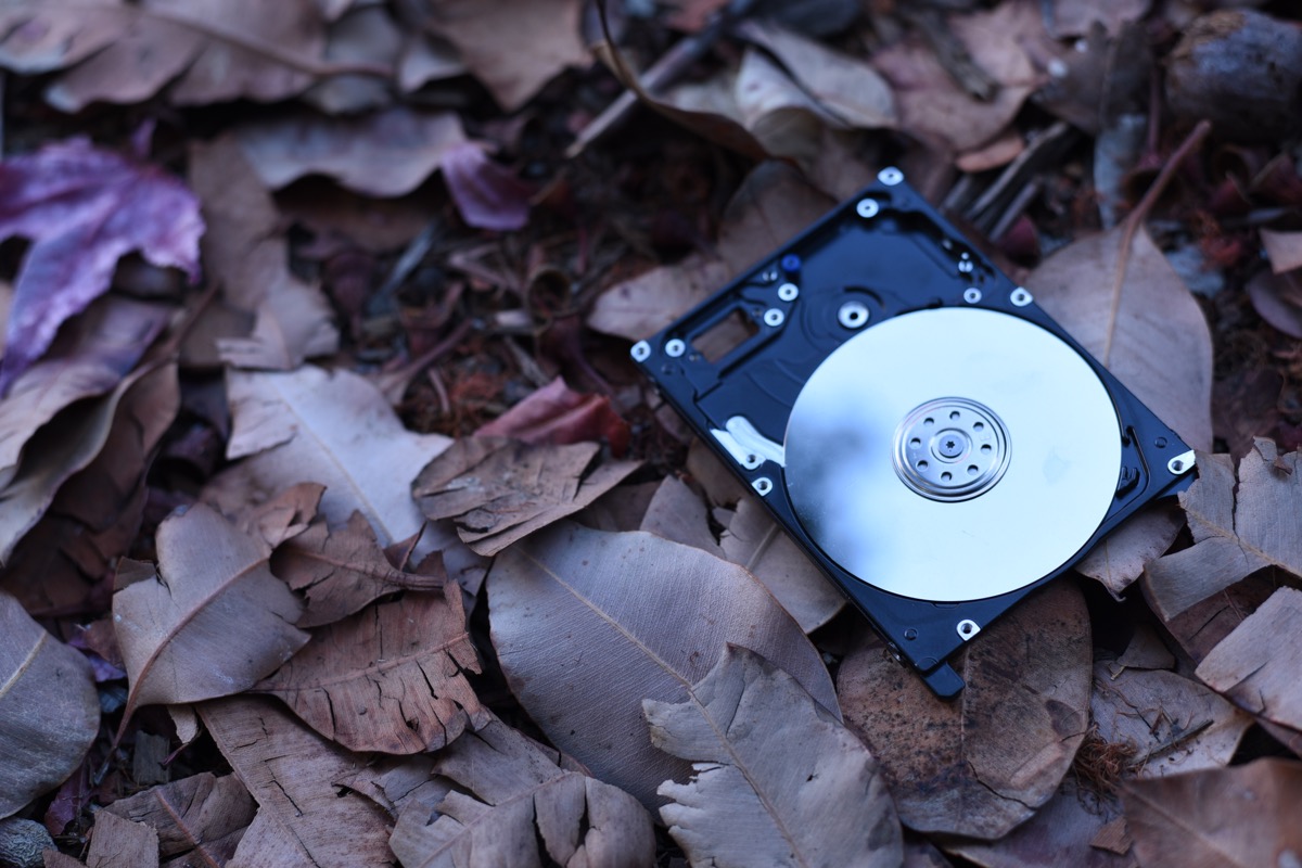
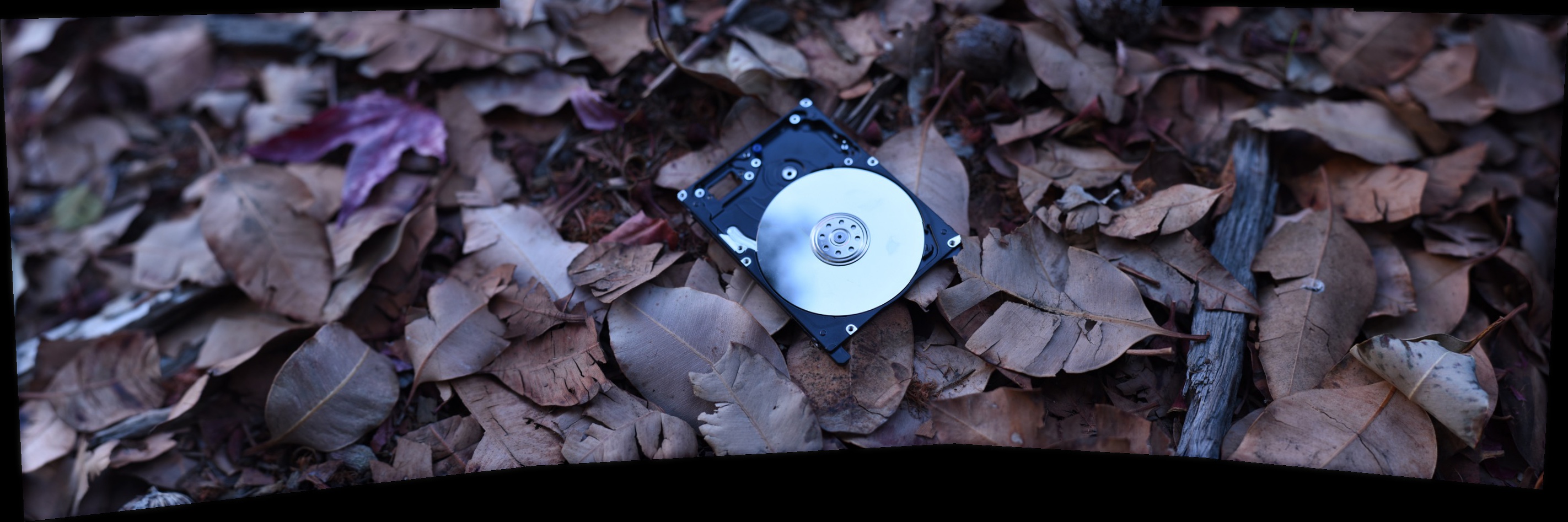
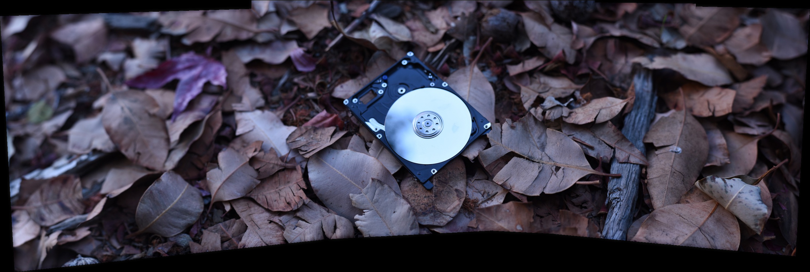
Here is another mosaic of the hard drive, but this time it is on the ground.
I wrote a function to project points onto a cylinder (cylindrical projection), and another function to do the inverse cylindrical projection.
The goal of this section was to enable support for very wide panoramas. When you have only 3 images, you can compute homographies between adjacent pairs directly. When you have 4 or more images, you need to multiply matrices together to get a homography matrix between 2 non-adjacent images. So, the images toward the edge of the panorama end up getting very stretched and very large (my computer runs out of memory).
One way to fix this is to use cylindrical projection. Instead of acting as a wide angle camera with a flat image plane, the cylindrical projection panorama pretends that the input images can be warped onto the inner surface of a cylinder, and then you can get the resulting image by peeling off the surface of the cylinder, like wrapping paper or tin foil. So, I used my inverse cylindrical projection function in order to do the image interpolation, and I used the regular cylindrical projection function to translate the annotated keypoints. Then, I used my regular projection warping code to morph the images together (I should have been able to use a translation instead of a projective transformation, but I didn't hold the camera exactly still when I took these photos).
This was just a test image to get a sense of what the cylindrical projection was doing.
I originally took a bunch of pictures in a 360° rotation, because I wanted to do the 360° interactive image, but I realized that I didn't have the patience to label so many images. Maybe I'll try that part in Part B after we have automatic annotation. But for now, I just took 5 of these images (from 1 corner) and used them in a panorama with cylindrical projection.
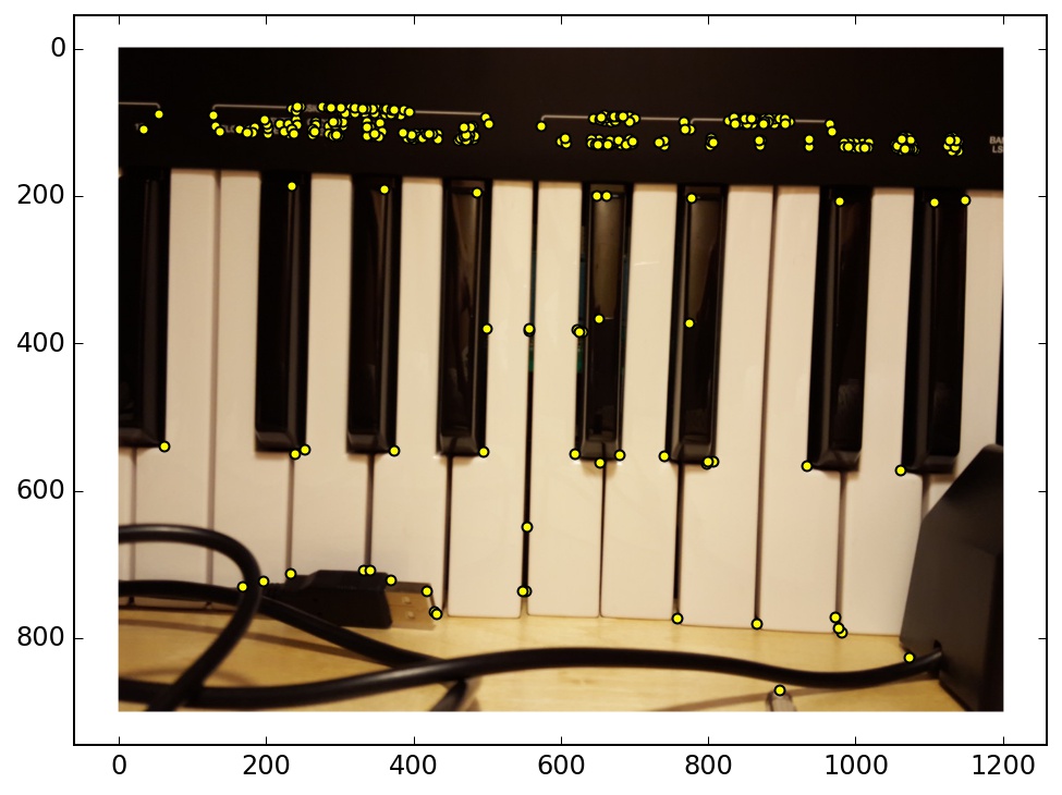
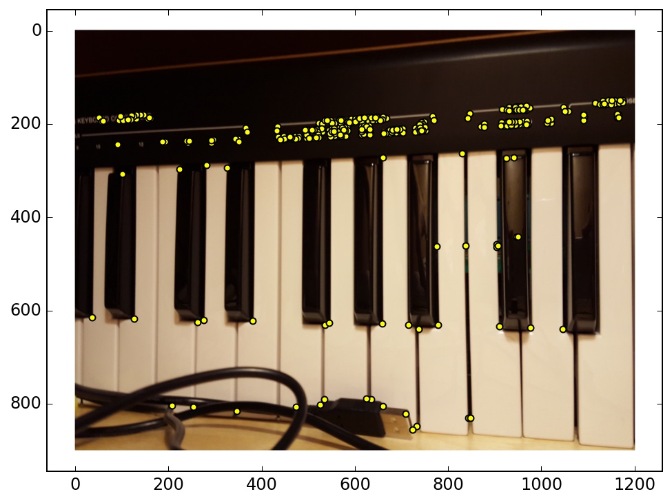
I used the Harris corner detector and non-maximum suppression to identify corners in an image. This was accomplished by the code that was given in the project spec. I also implemented adaptive non-maximal suppression, as outlined in the Brown et al paper.
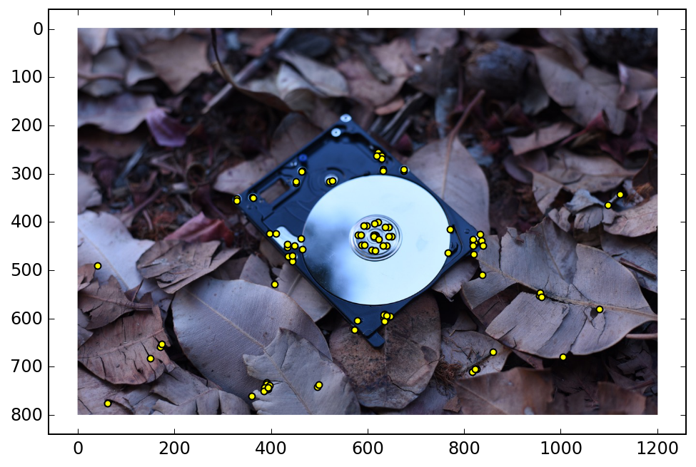
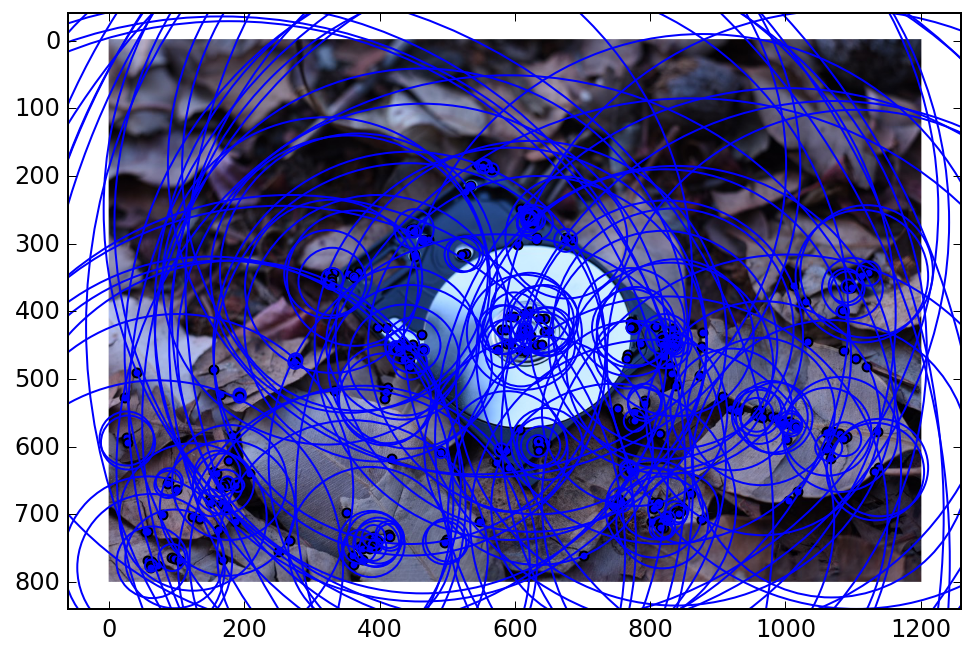
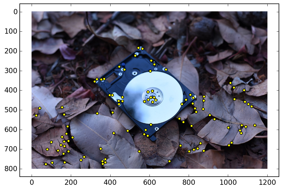
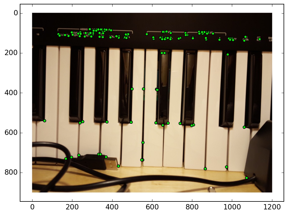
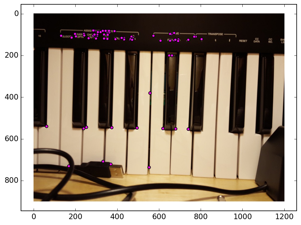
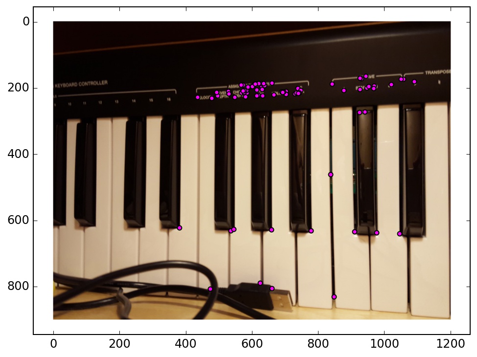
Adaptive non-maximal suppression was accomplished by computing a radius R(p) for each point p, which corresponds to the distance to the nearest neighbor that has a greater Harris value. I tweaked my algorthm to use a robustness constant, crobust = 0.9. I visualized this radius value by plotting circles that correspond to the size of the radius for each point. There are 50 corners in both the normal algorithm’s output and the adaptive algorithm’s output, but the adaptive algorithm’s output has a more uniform spread of points. When I actually put together the homographies, I used 300 corners instead of 50.
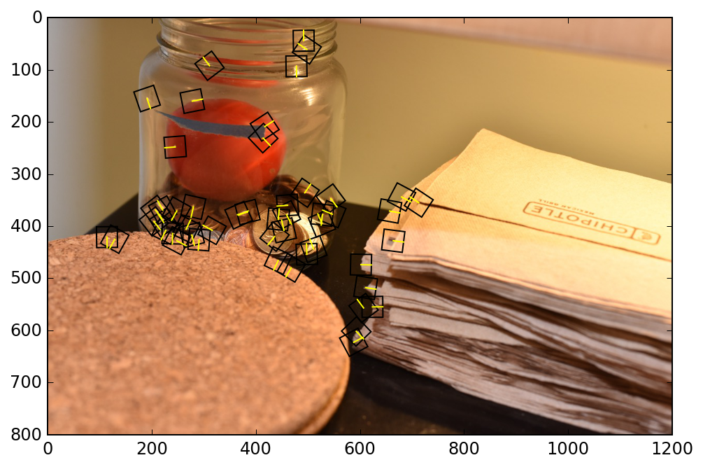
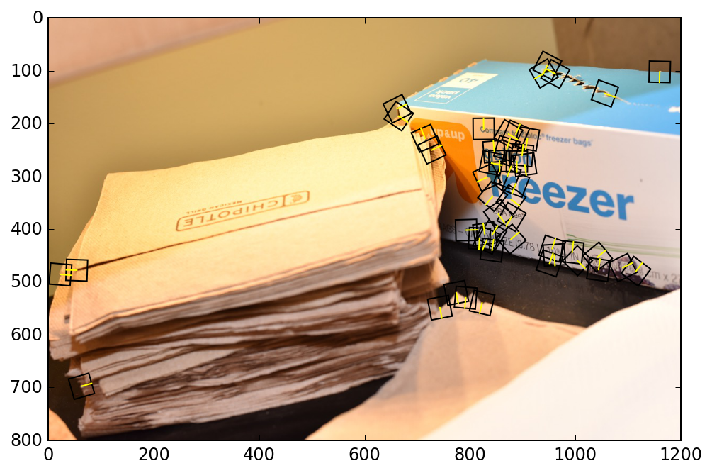
I then extracted 40x40 patches of pixels around the corner points that I identified previously. I used a 2D rotation matrix and linear interpolation to align each image patch with the gradient direction at that corner (some extra care must be taken to support a full 360° range of gradients). I used a Gaussian blur filter to smooth out the gradients. Corners that were too close to the image edge are disqualified. Each image patch is downsampled by a factor of 5 to create 8x8 corner feature descriptors. I normalized each feature descriptor to unit variance and zero mean.
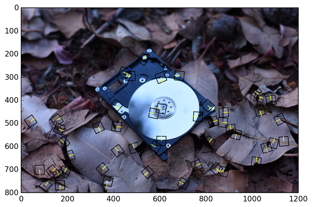
In this visualization of the corners, the yellow line in each square represents the gradient.
For each feature in the first image, I compute an error measure for the 1st and 2nd nearest neighbor features in the second image. I use the ratio of these 2 errors to throw out some likely false matches immediately (my threshold is set to 0.4). Then, I further reduce my feature matchings using RANSAC. I run the RANSAC algorithm for 10000 iterations for each matching. In each iteration, 4 random points are chosen and used to compute a homography.Then, I transform all the corner positions of the first image with this homography, and see which of them land close to their nearest neighbor feature in the second image. I use the squared euclidean distance to gauge “nearness”, and I threshold this at 3. After 10000 iterations, I use the set from the iteration that contained the most inliers, and I compute a homography using all of those points with the least squares method.

My automatic mosaics worked for the most part. Here are some examples where it succeeded, and one example where it did not.
The result of this example was almost identical between the manual and automatic mosaics.
There actually is a noticeable difference between the automatic and manual alignment in this example. However, both of them look pretty good, surprisingly.
In this case, the automatic stitching dropped the left-most image altogether. This is because it only found 3 inliers in the maximum RANSAC group, which was not enough to compute the homography. This might be because of the lack of corners in the first image, and this problem could potentially fixed if I changed the feature scale or tweaked some of the thresholds.
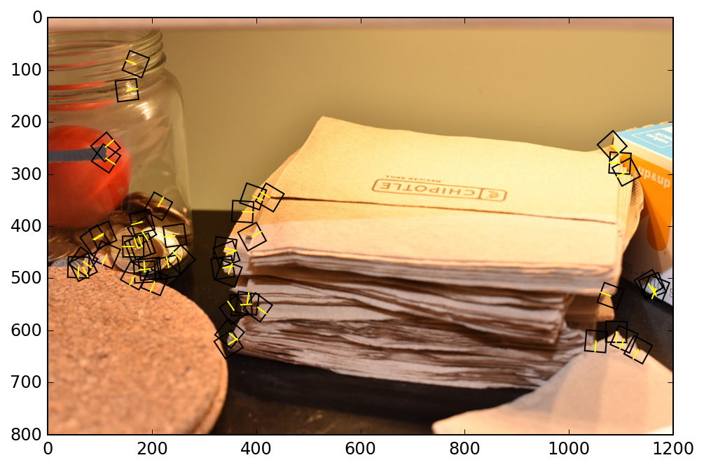
My features are supposed to be rotation invariant, so I tried rotating the camera while taking the panorama (trickier than it sounds). The result is the ability to stitch rotated mosaics automatically.
Here is a visualization of the rotated features. Notice that the rotation follows the rotation of the objects in the image, which helps the algorithm stitch this together.
At the beginning, I had a bug in my code where my rotated interpolation matrix was accidentally rotating in the opposite direction. Nonetheless, RANSAC was able to still correctly piece together the images in most cases, which was pretty impressive!